5. Methods#
methods implements function and modules DC-resistivity, EM, and Hydrogeological parameters calculations.
For the first release three main methods are implemented:
- DC-Resistivity method
DC-resistivity methods are cheaper and fast, especially the ERP and VES, the DC methods are the most used in developing countries for GWE. They are the most preferred methods to stay on the project schedule. Furthermore, from the DC-Profiling method implemented in watex from module electrical, the relevant appropriate features are extracted such as the conductive zone and the best position point for drilling [3].
- EM method
The method implemented in watex mainly focused on short periods, especially the Natural Source Audio-frequency Magnetotellurics (NSAMT) data. Indeed, the NSAMT is one of the EM methods occasionally found in GWE because it has some advantages compared to other geophysical short-period methods ([1], [4], [7], [11]). Unfortunately, NSAMT data suffers from frequency ranges with little or no signal in the “attenuation band” also known as the “dead band” [2].
watexworks around this issue by recovering the loss or weak signal due to man-made noise (human activities, existence of factories near the survey sites, power lines, etc) and updating new tensors. It also provides efficient filters to correct the tensors influenced by these noises, especially at a frequency in the range above 1 kHz.
- Hydrogeology method
it focuses on computing hydrogeology parameters such as permeability coefficient k, finding the aquifer group similarities, and managing the logging data indispensable in hydrogeological exploration ([6],[8]_). Genuinely, logging technology distinguishes the properties of rock and fluid by measuring the physical property of heat, sound, and electricity in the borehole compared to other geophysical methods ([5], 10]_). Thanks to the mixture learning strategy (MXS) implemented by watex, the combination of both methods infers the relationship between the logging data and the hydrogeological parameters thereby minimizing the numerous pumping test failures and reducing the useless boreholes.
5.1. DC-Resistivity: electrical#
For non-specialized users about the DC-resistivity methods especially the ERP and VES methods, it is suggested to take five-minutes reading to undertand the DC-methods before getting started with.
The electrical is composed of multiples DC readings prefixed par the DC as the names of the methods (DCProfiling,
DCSounding and single DC reading classes (ResistivityProfiling and VerticalSounding).
The latter offers supplemental plot functions whereas the former does not.
5.1.1. Resistivity Profiling (ERP): ResistivityProfiling#
ResistivityProfiling deals with single Electrical Resistivity Profiling (ERP).
The method is composed of station, resistivity data, and/or coordinates of measurements. Refer to Datasets for further details.
As an example, we will make samples of 100 measurements using the function make_erp() and compute the DC -electrical parameters for flow rate prediction [3].
The summary() recaps all the prediction parameters.
Note
For demonstration, I assume that the drilling is performed at station 5(S05) on the survey line, i.e the DC parameters are computed at that station. However, if the station is not specified, the algorithm will find the best conductive zone based on the resistivity values and will store the value in attribute sves_ (position to make a drill). The auto-detection can be used when users need to propose a place to make a drill. Note that for a real case study, it is recommended to specify the station where the drilling operation was performed through the parameter station. For instance, automatic drilling location detection can predict a station located in a marsh area that is not a suitable place for making a drill. Therefore, to avoid any misinterpretation due to the complexity of the geological area, it is useful to provide the station position. The following examples illustrate the aforementioned details:
Compute the DC parameters and plot the conductive zone at stations S5
>>> from watex.datasets import make_erp
>>> erp_data = make_erp ( n_stations =100 ).frame
>>> erp_data.head(3)
   station  longitude  latitude        easting    northing  resistivity
0      0.0 -13.488511  0.000997  668210.580864  110.183287   233.090909
1     20.0 -13.488511  0.000997  668210.581026  110.183416    81.727273
2     40.0 -13.488511  0.000997  668210.581188  110.183544   202.818182
>>> from watex.methods import ResistivityProfiling
>>> erpo = ResistivityProfiling (station ='S05').fit(erp_data )
>>> erpo.power_
60
>>> erpo.sfi_
array([1.048])
>>> erpo.conductive_zone_
array([202.8182, 212.9091, 656.9091, 132.1818, 374.3636, 808.2727, 979.8182])
>>> erpo.summary (return_table=True )
        dipole  longitude  latitude  ...  shape  type       sfi
station                               ...
S005         10  -13.48851  0.000997  ...      C    PC  1.047981
>>> erpo.plotAnomaly(style ='classic') # outputs the following figure

Compute the DC parameters and plot the conductive zone using the automatic-detection
>>> from watex.methods import ResistivityProfiling
>>> erpo = ResistivityProfiling (auto=True).fit(erp_data ).summary(keep_params=True)
>>> # Note that if `auto` is not set to True when the station is not given,
>>> # it will be triggered by force and raising a warning message
>>> erpo.table_
   power   magnitude shape type       sfi
0     60  968.727273     V   PC  1.331279
>>> erpo.plotAnomaly (style ='classic')
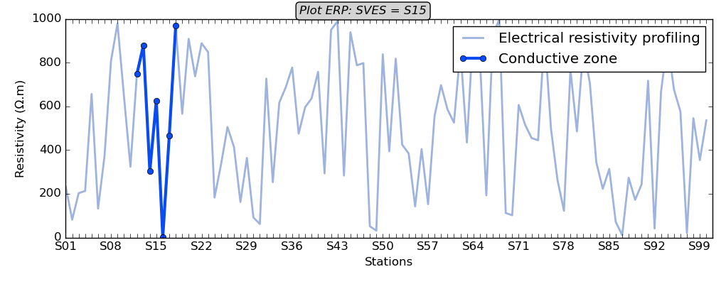
Here, the automatic detection specifies the best point for making a drill to S15 with its prediction
parameters summarized in the table_.
5.1.2. Vertical Sounding (VES): VerticalSounding#
VerticalSounding is carried out to speculate about the
existence of a fracture zone and the layer thicknesses. Commonly, it comes as a supplement
method to ERP after selecting the best conductive zone. The main data that compose the VES
are AB and resistivity. The MN is not compulsory. Note that by convention AB is AB/2 in meters
and the resistivity is preferably expressed in \(\Omega.m\). In the following example, we will generate
samples of 31 measurements in deeper using the function make_ves().
Furthermore, VerticalSounding has a search parameter which is very useful. Indeed,
the parameter passed to the above class is implemented to find water outside of the pollution. Usually, when exploring
deeper using the VES, we are looking for groundwater in the fractured rock that is outside the anthropic
pollution [12]. Thus the search parameter indicates where the search for the fracture zone in
deeper must start. For instance, search=45 tells the algorithm to search or start detecting the
fracture zone from 45m to deeper.
Compute the ohmic-area OhmS prediction parameters and plot the searching fracture zone
>>> from watex.datasets import make_ves
>>> ves_data = make_ves ( seed=42, iorder =5 ).frame
>>> ves_data.tail (7)
           AB    MN  resistivity
24   61.0   5.0   434.728606
25   65.0   5.0   429.921368
26   69.0  10.0   420.808772
27   79.0  10.0   374.251687
28   89.0  10.0   320.386412
29   99.0  10.0   372.161240
30  109.0  10.0   770.101644
>>> from watex.methods import VerticalSounding
>>> veso = VerticalSounding (search = 60 ).fit(ves_data )
>>> veso.ohmic_area_
867.2945999304986
>>> veso.fractured_zone_
array([ 61.,  65.,  69.,  79.,  89.,  99., 109.])
>>> veso.fractured_zone_resistivity_
array([491.7705, 423.5979, 371.0891, 308.3456, 343.5002, 476.5529,
           707.5036])
>>> veso.plotOhmicArea (fbtw=True , style ='classic')

Here the ohmic-area zone is hatched (fill_between) with a value equal to \(867.3 \Omega.m^2\). The summarized parameters can be collected using:
>>> veso.summary(return_table=True )
                 AB    MN   arrangememt utm_zone  ... search max_depth  ohmic_area  nareas
area                                      ...
None  200.0  20.0  schlumberger     None  ...     60     109.0    867.2946       1
5.1.3. DC-Profiling: DCProfiling#
DCProfiling reads a collection of DC-resistivity profiling data.
It computes electrical profiling parameters and store data in a line object where each line
is ResistivityProfiling object. For instance, the expected drilling
location point and its resistivity value for two survey lines ( line1 and line2) can be fetched as:
>>> <object>.line1.sves_ ; <object>.line1.sves_resistivity_
>>> <object>.line2.sves_ ; <object>.line2.sves_resistivity_
For further details about the parameters explanations, click
on DCProfiling . The following examples give a real
example of data collected and stored in the software data/erp directory.
Get DC -resistivity profiling from the individual ERP data
>>> from watex.datasets import make_erp
>>> from watex.methods import DCProfiling
>>> dcpo= DCProfiling(auto=True) # auto detection
>>> data1 = make_erp ( n_stations =100 ).frame
>>> data2 = make_erp ( n_stations =70 , max_rho = 1e4).frame
>>> data3 = make_erp (n_stations = 150, min_rho=1e2, max_rho=1e5 ).frame
>>> dcpo.fit(data1, data3, data3 )
>>> dcpo.nlines_ # number of lines read
    dc-erp: 100%|##################################| 3/3 [00:00<00:00, 190.98B/s]
    3
>>> dcpo.sves_ # the best automatic conductive zone
Out[417]: array(['S036', 'S097', 'S097'], dtype=object)
>>> dcpo.line1.sves_ # line 1 best drilling point
    'S036'
    >>> dcpo.line2.sfi_ # pseudo-fracturing index at the best drilling point
    1.3068009325282002
    >>> dcpo.line3.conductive_zone_ # the conductize zone of position of the line3
    array([37646.3087, 61112.7517, 97318.1208,   100.    , 54408.0537,
               98659.0604, 26248.3221])
    >>> dcpo.summary() # summarized the computed parameters
               dipole  longitude  latitude  ...  shape  type       sfi
    line1      10  -13.48851  0.000997  ...      C    PC  1.265274
    line2      10  -13.48851  0.000997  ...      M    PC  1.306801
    line3      10  -13.48851  0.000997  ...      M    PC  1.306801
Read a collection of ERP data in excel sheets
>>> datapath = 'data/erp'
    >>> dcpo= DCProfiling(auto=True) #
>>> dcpo.read_sheets=True
>>> dcpo.fit(datapath, force =True) # force the reading i.e transform the raw data to a selector ERP.
    dc-erp: 100%|##################################| 4/4 [00:00<00:00, 257.36B/s]
    DCProfiling(AB= 200.0, MN= 20.0, arrangememt= schlumberger, ... , auto= True, keep_params= False, read_sheets= True)
>>> dcpo.nlines_  # getting the number of survey lines to read successfully
4
    >>> dcpo.line2.sves_resistivity_
    93
>>> dcpo.sves_ # stations of the best conductive zone
array(['S017', 'S001', 'S000', 'S036'], dtype=object)
>>> dcpo.sves_resistivities_ # the lower conductive resistivities
array([  80.,   93., 1101.,  500.])
>>> dcpo.powers_
array([ 50.,  40.,  30., 180.])
    >>> dcpo.survey_names_  # name of the four lines read
    ['sheet1', 'l11_gbalo', 'sheet2', 'sheet3']
5.1.4. DC-Sounding: DCSounding#
DCSounding reads a collection of VES data and stores
the computed predictor in a VerticalSounding object.
Contrary to DCProfiling , data is stored in site object
not in line. Retrieving data from each DC-sounding site follow the naming below:
>>> <object>.site<number>.<:attr:`~.VerticalSounding.<attr>_`
For instance to fetch the DC-sounding data position and the resistivity in depth of the fractured zone for the first site, it should be:
>>> <object>.site1.fractured_zone_
>>> <object>.site1.fractured_zone_resistivity_
For parameters explanation, refer to DCSounding instead. The
following examples will illustrate the literature above:
Read a single DC Electrical Sounding file
>>> from watex.methods.electrical import DCSounding
>>> dcvo= DCSounding ()
>>> dcvo.search = 30. # start detecting the fracture zone from 30m depth.
>>> dcvo.fit('data/ves/ves_gbalo.xlsx')
    dc-ves: 100%|###################################| 1/1 [00:00<00:00, 49.00B/s]
>>> dcvo.ohmic_areas_
array([523.25458506])
>>> dcvo.site1.fractured_zone_ # show the positions of the fracture zone
array([ 28.,  32.,  36.,  40.,  45.,  50.,  55.,  60.,  70.,  80.,  90.,
       100.])
>>> dcvo.site1.fractured_zone_resistivity_
array([ 66.1963,  67.5732,  69.2663,  71.2754,  74.2315,  77.6814,
    81.6254,  86.0633,  96.4209, 108.7543, 123.0635, 139.3486])
Read Multiple Sounding files from sheets
    >>> dcvo= DCSounding ()
    >>> dcvo.fit('data/ves')        # read the ves data in directory
    >>> dcvo.survey_names_          # survey names successfully read
    ['ves_gbalo', 'ves_gbalo', 'ves_gbalo', 'ves_gbalo_unique']
>>> dcvo.ohmic_areas_
    array([ 268.0877,  268.0877, 1183.3641])
    >>> dcvo.nareas_
    array([2., 2., 2.])
>>> dcvo.summary()
                      AB    MN   arrangememt  ... max_depth   ohmic_area nareas
    site1  200.0  20.0  schlumberger  ...       100   268.087715      2
    site2  200.0  20.0  schlumberger  ...       100   268.087715      2
    site3  200.0  20.0  schlumberger  ...       100  1183.364102      2
5.2. EM: em#
em module is related to a few meter exploration in the case of groundwater
exploration(GWE). The module provides some basic processing steps for EMAP data filtering
and removing noises. Commonly the method mostly used in groundwater exploration is the audio-magnetotelluric because of
the shortest frequency and rapid executions. Furthermore, we can also list some other advantages
such as:
is useful for imaging both deep geologic structure and near-surface geology and can provide significant details.
includes a backpack portable system that allows for use in difficult terrain.
the technique requires no high-voltage electrodes, and logistics are relatively easy to support in the field. Stations can be acquired almost anywhere and can be placed any distance apart. This allows for large-scale regional reconnaissance exploration or detailed surveys of local geology and has no environmental impact
Note
Note that for deep implementation especially for long-period data, or exploring a large scale of EM/AMT data
processing, it is recommended to visit other the package pycsamt , MTpy, razorback or MTnet website.
watex can also read EDI objects created from the first both packages.
Note that the EMAP inherits from EM class. When EDI data is passed
to EM fit() method, each Edi-file is considered as an EM object, and attributes
are wrapped and recomputed such the coordinates, ids sites, frequency and reference frequency. EDI files can also rewrite accordingly
using the EM rewrite() method. The latter gives many options for EDI outputs. Refer to
rewrite() for further details about parameters.
For the whole examples, let’s fetch 21 examples of EDI files stored in load_edis().
>>> from watex.datasets import load_edis
>>> from watex.methods import EM
>>> edi= load_edis (samples =21 )
>>> edi.frame.site[:7].values
array(['e.E00', 'e.E01', 'e.E02', 'e.E03', 'e.E04', 'e.E05', 'e.E06'],dtype=object)
>>> edi.frame.edi [:7].values
array([Edi( verbose=0 ), Edi( verbose=0 ), Edi( verbose=0 ),
           Edi( verbose=0 ), Edi( verbose=0 ), Edi( verbose=0 ),
           Edi( verbose=0 )], dtype=object)
>>> edi.frame.columns
Index(['name', 'longitude', 'edi', 'site', 'latitude', 'id'], dtype='object')
>>> edi_data = edi.frame.edi.values
>>> e= EM().fit(edi_data )
>>> e.freqs_ # from higher to lower frequency
array([58800.  , 52128.64, 46214.21, 40970.82, 36322.34, 32201.26,
           28547.76, 25308.77, 22437.28, 19891.58, 17634.71, 15633.91,
           13860.11, 12287.56, 10893.43,  9657.48,  8561.76,  7590.36,
                6729.17,  5965.69,  5288.83,  4688.77,  4156.79,  3685.16,
                3267.05,  2896.38,  2567.76,  2276.42,  2018.14,  1789.17,
                1586.17,  1406.21,  1246.66,  1105.22,   979.82,   868.65,
                 770.1 ,   682.72,   605.26,   536.59,   475.71,   421.74,
                 373.89,   331.47,   293.86,   260.52,   230.96,   204.76,
                 181.52,   160.93,   142.67,   126.48,   112.13,    99.41])
>>> e.refreq_ # reference frequency
58800.0
Note that the tensor components z (impedances), resistivity, and phases are stored in a three-dimensional array of (n_frequency, 2, 2 ) for xx, xy , yx and yy. It is possible to get the corresponding tensor component in the two-dimensional array from the method make2d(). By default make2d() outputs resistivity components xy. Rather than deleting the missing tensors, they are kept in the tensor as NaN signal and should be used for corrections. As mentioned above, most short-period EM specially NSAMT suffers from the lower and missing signal. Deleting many tensors will yield poor data processing. As a result, a misinterpretation should be done for the location of the drilling operations. Refer to the method (make2d()) documentation for more details.
>>> zxy = e.make2d (out = 'zxy') # out complex
>>> zxy.shape
(54, 21)
The code snippets below show a concrete example of data composed of weak signal and missing tensor located directory
>>> from watex.methods.em import EM
>>> edipath ='data/edis'
>>> emObjs= EM().fit(edipath)
>>> phyx = EM().make2d ('phaseyx')
>>> phyx  # missing tensor a refered as NaN values.
array([[ 26.42546593,  32.71066454,  30.9222746 ],
           [ 44.25990541,  40.77911136,  41.0339148 ],
           ...
           [ 37.66594686,  33.03375863,  35.75420802],
           [         nan,          nan,  44.04498791]])
>>> phyx.shape
(55, 3)
>>> # get the real number of the yy components of tensor z
>>> zyy_r = make2d (ediObjs, 'zyx', kind ='real')
array([[ 4165.6   ,  8665.64  ,  5285.47  ],
           [ 7072.81  , 11663.1   ,  6900.33  ],
           ...
           [   90.7099,   119.505 ,   122.343 ],
           [       nan,        nan,    88.0624]])
>>> # get the resistivity error of component 'xy'
>>> resxy_err = EM.make2d ('resxy_err')
>>> resxy_err
array([[0.01329037, 0.02942557, 0.0176034 ],
           [0.0335909 , 0.05238863, 0.03111475],
           ...
           [3.33359942, 4.14684926, 4.38562271],
           [       nan,        nan, 4.35605603]])
>>> phyx.shape ,zyy_r.shape, resxy_err.shape
((55, 3), (55, 3), (55, 3))
5.2.1. Restoring tensors: zrestore()#
In the following, we will show some examples for restoring signal and processing EDI data using the EM EMAP
class. The signal recovery is ensured by the zrestore(). Before, the EDI quality data
can be analyzed using the qc() method. For instance:
>>> from watex.methods.em import EMAPProcess
>>> pobj = EMAPProcess().fit('data/edis')
>>> f = pobj.getfullfrequency ()
>>> # len(f)
>>> # 55 frequencies
>>> c,_ = pobj.qc ( tol = .6 ) # mean 60% to consider the data as representatives
>>> c  # the representative rate in the whole EDI- collection
0.95 # the whole data at all stations is safe to 95%.
>>> # now check the interpolated frequency
>>> c, freq_new  = pobj.qc ( tol=.6 , return_freq =True) # returns the interpolated frequency
If the quality is so poor, there is a possibility to remove the bad data using
the getValidTensors() method. Indeed the getValidTensors() method
analyzes the data and keeps the good ones. The goodness of the data depends on the threshold rate. For instance 50% means to c
onsider an impedance tensor ‘z’ valid if the quality control shows at least that score at each frequency of all stations. For example:
>>> from watex.methods import EMAP
>>> pObj = EMAP().fit('data/edis')
>>> f= pObj.freqs_
>>> len(f)
55
>>> zObjs_soft = pObj.getValidTensors (tol= 0.3, option='None' ) # None doesn't export EDI-file
>>> len(zObjs_soft[0]._freq) # suppress 3 tensor data
52
>>> zObjs_hard  = pObj.getValidTensors( tol = 0.6 )
>>> len(zObjs_hard[0]._freq)  # suppress only two
53
Note
The sample of EDI data stored in load_edis() is already preprocessed data so it is not useful for a
software demonstration. Rather, we use the concrete data/edis/ . However, the data is not available in the software repository data/edis
and can be collected upon request.
The tensors recovering can be operated as :
>>> from watex.methods.em import EMAP
>>> path2edi = 'data/edis'
>>> pObjs= EMAP().fit(path2edi)
>>> # One can specify the frequency buffer like the example below, however
>>> # it is not necessary at least there is a specific reason to fix the frequencies beforehand.
>>> buffer = [1.45000e+04,1.11500e+01]
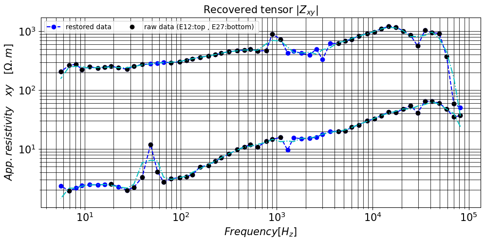
>>> zobjs_b = pObjs.zrestore(
# buffer = buffer
)
zobjs_b is a new tensor recovered in (n_frequency, 2,2 ) dimensions. The following output gives a real example of recovery tensors of the raw data ( containing missing tensors) of stations E12 and E27 collected at all frequencies. The blue dot markers are the tensor data recovered at the missing frequency signals. Note that the recovery tensor is used to (re)compute the apparent resistivity.
5.2.2. Filtering tensors: ama(), flma() & tma()#
After recovering the signal, the latter exhibits a field strength amplitude for the next processing step like filtering. watex implements three filterings linked to the EMAP class such as the adaptative moving average (AMA), the fixed-dipole length moving average (FLMA), and the trimming-moving average (TMA). Note that when using the AMA filter, the c parameter is a window-width expansion factor that must be input to the filter adaptation process to control the roll-off characteristics of the applied Hanning window [13]. Here is an illustration:
>>> import numpy as np
>>> import matplotlib.pyplot as plt
>>> from watex.methods import EMAP
>>> from watex.datasets import fetch_data # load_edis
>>> e= fetch_data ('edis', samples =21, key='*' ) #"*" to fetch all columns of edi data
>>> # the above code is the same as
>>> # e= load_edis (samples =21 , key='*')
>>> edi_data = e.frame.edi.values
>>> pobj= EMAP(window_size =5, component='yx', c= 2, out='srho').fit( edi_data ) # 'srho' for static resistivity correction'
>>> resyx = pobj.make2d ('resyx')
>>> res_ama = pobj.ama()
>>> res_flma = pobj.flma ()
>>> res_tma = pobj.tma ()
>>> x_stations = np.arange (len(e.frame.site ))
>>> plt.xticks (x_stations , list (e.frame.id))
>>> # corrected Edi at station S00
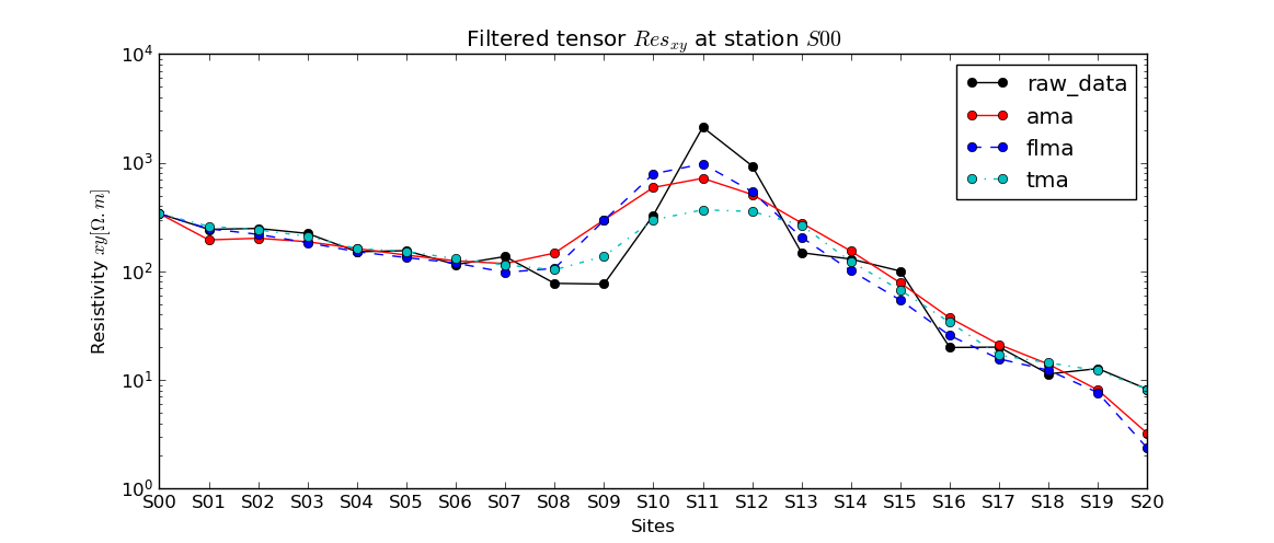
>>> plt.semilogy (x_stations, resyx[0, :] , 'ok-', label ='raw_data' )
>>> plt.semilogy(x_stations, res_ama[0, :] ,'or-', label ='ama')
>>> plt.semilogy(x_stations, res_flma [0, :], 'ob--', label ='flma')
>>> plt.semilogy(x_stations, res_tma[0, :] , 'oc-.', label ='tma')
>>> plt.title ("Filtered tensor $Res_{xy}$ at station $S00$")
>>> plt.legend ()
>>> plt.xlabel ("Sites") ; plt.ylabel ("Resistivity ${xy}[\Omega.m]$")
>>> plt.style.use ('classic')
The following picture shows the different filters applied on the first station S00.
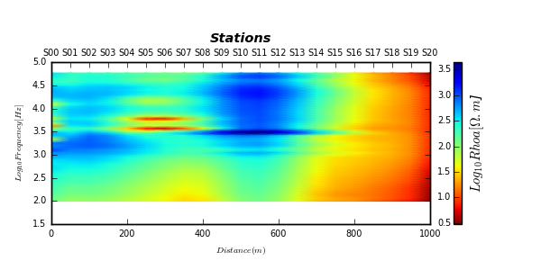
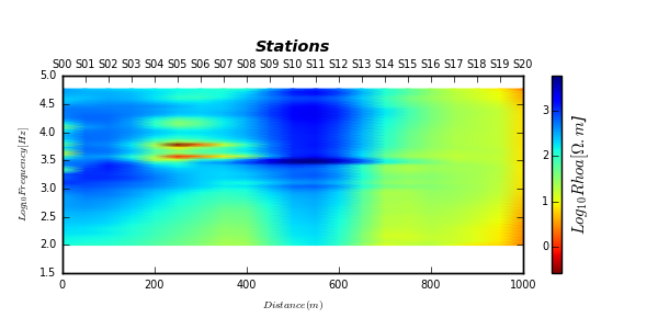
The next figures show the filtered data in a two-dimensional layout. The plot is handled using the TPlot class.
The code snippets are given below:
>>> from watex.view.plot import TPlot
>>> from watex.datasets import load_edis
>>> # get some 3 samples of EDI for demo
>>> # customize plot by adding plot_kws
>>> plot_kws = dict( ylabel = '$Log_{10}Frequency [Hz]$',
                                        xlabel = '$Distance(m)$',
                                        cb_label = '$Log_{10}Rhoa[\Omega.m$]',
                                        fig_size =(6, 3),
                                        font_size =7.
                                        )
>>> t= TPlot(component='yx', **plot_kws ).fit(edi_data)
>>> # plot recovery2d using the log10 resistivity
>>> t.plot_tensor2d (to_log10=True) # for raw tensor
>>> t.plot_ctensor2d (to_log10=True)
>>> t.plot_ctensor2d (to_log10=True, ffilter='flma')
>>> t.plot_ctensor2d (to_log10=True, ffilter='ama')
Noise data vs filtered data (AMA, FLMA and TMA) ?
Noise data
AMA
FLMA
TMA


Note, there are many other functions in em that can be implemented. One of them is
the method exportedis() that exports the new tensor (new_Z) for modeling
after updating tensor using the decorator _zupdate by triggering
the option parameter to write.
5.3. Hydrogeology: hydro#
hydro deals with the hydrogeological parameters calculations of aquifers.
These parameters are essential and crucial in the designing and construction progress of geotechnical
engineering and groundwater dewatering, which are directly related to the reliability of these parameters.
In the following, it is useful to remember the hydrogeological attribute definition below:
- aqname
Name of aquifer group column. aqname allows retrieving the aquifer group arr_aq value in a specific data frame. Commonly`aqname` needs to be supplied when a data frame is passed as a positional or keyword argument. Note that it is not mandatory to have a group of the aquifer in the log data. It is needed only if the label similarity needs to be calculated.
- sname
Name of the column in the data frame that contains the strata values. Don’t confuse sname with stratum which is the name of the valid layer/rock in the array/Series of strata.
- z
An array of depth or a pandas series that contains the depth values. A two-dimensional array or more is not allowed. However when z is given as a dataframe and zname is not supplied, an error raises since zname is used to fetch and overwrite z from the data frame.
- zname
Name of depth columns. zname allows retrieving the depth column in a data frame. If an integer is passed, it assumes the index of the data frame fits the depth column. Integer value must not be out of the data frame size along axis 1. Commonly zname needs to be supplied when a data frame is passed to a function argument.
- kname
Name of permeability coefficient columns. kname allows retrieving the permeability coefficient ‘k’ in a specific data frame. If an integer is passed, it assumes the index of the data frame fits the k columns. Note that the integer value must not be out of the data frame size along axis 1. Commonly kname needs to be supplied when a data frame is passed as a positional or keyword argument.
- k
An array of permeability coefficient k or a pandas series that contains the k values. A two-dimensional array or more is not allowed. However, when k passes as a data frame and kname is not supplied, an error raises since kname is used to retrieve k values from the data frame and overwritten it.
Here is data that composes the hydro-geophysical dataset (HGDS):
>>> from watex.datasets import load_hlogs
>>> load_hlogs ().frame.columns
Index(['hole_id', 'depth_top', 'depth_bottom', 'strata_name', 'rock_name',
           'layer_thickness', 'resistivity', 'gamma_gamma', 'natural_gamma', 'sp',
           'short_distance_gamma', 'well_diameter', 'aquifer_group',
           'pumping_level', 'aquifer_thickness', 'hole_depth_before_pumping',
           'hole_depth_after_pumping', 'hole_depth_loss', 'depth_starting_pumping',
           'pumping_depth_at_the_end', 'pumping_depth', 'section_aperture', 'k',
           'kp', 'r', 'rp', 'remark'],
          dtype='object')
5.3.1. Aquifer section: AqSection#
AqSection get the section of each aquifer from the HGDS. For further details about the
hydro-dataframe, read the documentation of the load_hlogs(). Indeed, the unique
section ‘upper’ and ‘lower’ is the valid range of the whole data to consider as valid data. Indeed, the aquifer
section computing is necessary to shrink the data of the whole boreholes. Mostly the data from the section is
considered valid data as the predictor:math:X_r. Out of the range of the aquifers section, data can be discarded
or compressed to the top \(X_r\). Refer to hydroutils for additional details.
Here is an example of computing a section from a single borehole data H502 (default):
>>> from watex.datasets import load_hlogs
>>> from watex.methods import AqSection
>>> h =load_hlogs (key='h502')
>>> ao = AqSection (aqname ='aquifer_group', kname = 'k', zname ='depth_top').fit(h.frame)
>>> ao.findSection ()
[197.12, 340.35]
In the above example, the valid section of the aquifer is found between 197.12 and 340.35 meters deep.
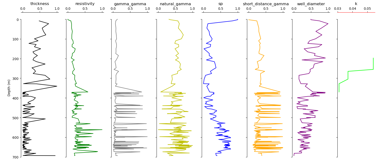
5.3.2. Logging: Logging#
Logging class deals with the numerical values of HGDS that compose the
predictor \(X\). If categorical values are found in the logging dataset, they should be discarded.
Here is an example of plotting the logging data.
>>> from watex.datasets import load_hlogs
>>> from watex.methods.hydro import Logging
>>> # get the logging data
>>> h = load_hlogs ()
>>> h.feature_names
['hole_id',
 'depth_top',
 'depth_bottom',
 'strata_name',
 'rock_name',
 'layer_thickness',
 'resistivity',
 'gamma_gamma',
 'natural_gamma',
 'sp',
 'short_distance_gamma',
 'well_diameter']
>>> # we can fit to collect the valid logging data
>>> log= Logging(kname ='k', zname='depth_top' ).fit(h.frame[h.feature_names])
>>> log.feature_names_in_ # categorical features should be discarded.
... ['depth_top',
             'depth_bottom',
             'layer_thickness',
             'resistivity',
             'gamma_gamma',
             'natural_gamma',
             'sp',
             'short_distance_gamma',
             'well_diameter']
>>> log.plot ()
... Logging(zname= depth_top, kname= k, verbose= 0)
>>> # plot log including the target y
>>> log.plot (y = h.frame.k, draw_spines =(0, 7)) #first position
... Logging(zname= depth_top, kname= k, verbose= 0)
The figure below shows the following outputs. Note that the logging plot has many parameters to customize the plot. Refer to
plot_logging() for further details.
5.3.3. Mixture Learning Strategy (MXS): MXS#
MXS entails predicting the permeability coefficient k from the HGDS data. Note
that the dataset for predicting k comes with a lot of missing data in the target \(y\). This is obvious
since the k is strongly tied to the productive aquifer and is collected after the pumping test. Commonly the
pumping is performed if and only if the layer is an aquifer. To work around this issue and to predict k with an
optimal score, watex implements a new ML approach called MXS. The approach first predicts upstream the naïve group
of aquifers (NGA) s using the clustering algorithms such as K-Means and Hierarchical Agglomerative Clustering (HAC).
The HAC dendrogram is used to validate the number of clusters that fit the NGA as well as the silhouette and elbow
metrics using the K-Means. NGA assumes to be the main aquifer group in the area. Once the NGA is predicted, an MXS
target:math:y* is created by merging the NGA labels with the true label (valid k) in the target \(y\) following
criteria of label similarity computation using Bayesian evidential learning. The NGA labels are used to compensate
for the missing k in the target y. The new MXS target \(y*\) represents a full-strength target ready for
predicting k using the supervised learning algorithms. The case history implemented in the Hongliu coal mine with 11
boreholes has successfully given more than 80% of correct prediction of k using the SVM radial basis kernel ([3], [14]) and XGB.
Here are the following code snippets to achieve the results using a single borehole ‘h2601’. First, I fetch the logging data stored in the software for visualization to see what a sample of logging data looks likes:
>>> from watex.datasets import load_hlogs
>>> from watex.methods import Logging, MXS
>>> ho= load_hlogs ( key = 'h2601')
For the following, I drop the observation ‘remark’ in the test sample since there is no valid data:
>>> hdata = ho.frame.drop (columns ='remark')
Since we are both dealing with unsupervised learning and supervised learning, the problem is turned into a classification task by categorizing k using into three classes ( \(k1: 0 < k≤0.01 m/d\)) encoded to {1} , (\(k2: 0.01<k≤0.07 m/d\)) encoded to {2} and ( \(k3:k>0.07 m/d\)) encoded to {3} . This default classification can efficiently be performed by turning the default_func parameter to True, then the NGA labels can be predicted using:
>>> mo= MXS(n_groups= 3, kname ='k', aqname='aquifer_group').fit(hdata)
>>> yNGA = mo.predictNGA(return_label=True )
>>> ymxs = mo. makeyMXS(yNGA , categorize_k=True, default_func=True)
>>> # or ymxs = mo.predictNGA().makeyMXS(categorize_k=True, default_func=True)
Once the \(y*\) ( ymxs) is created, it can be encoded and use the modeling step enumerated in the first example for the supervising learning. The model training phase can be handled by the models via the module GridSearch or GrdiSearchMultiples for single-model training and multiple models training respectively. A real-world example of model training results using the XGB is given in the figure below. The plot can be ensured with the function
plot_learning_curves() from utils. The machine performance inspection can also be handled with the plotLearningInspection() function in view . For multiple inspections, use plotLearningInspections() instead. Note the <s> at the end of <“Inspection”>. Moreover, the sign (+)
is the optimal model with a tradeoff found between the bias and the variance, and below are the hyperparameters values of
selected models. For reproducing the model results, send the request for collecting the case history data.
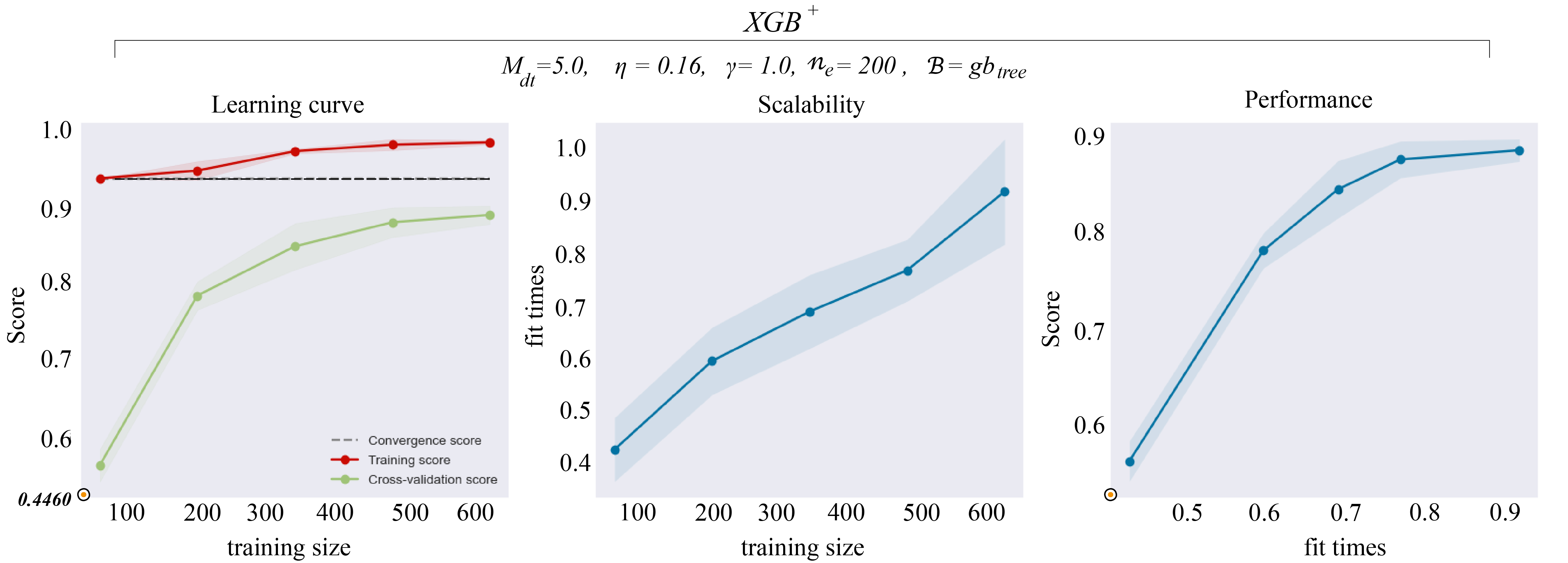
The left panel of the figure above is for the learning curve. The center panel is for the model scalability and the right panel is for the model performance. \(XGB^{+}\) paradigm finds out a good tradeoff between computation time and performance since it reaches its optimal performance with a relatively faster time. \(M_{dt}\): Maximum depth of trees. \(\eta\): Learning rate for boosting trees (between 0 and 1). \(\beta\) is the booster. It could be linear (Lin), tree (Tree), or Dropouts with multiple Additive Regression Trees (DART). \(\eta_e\): the number of the rounds/estimators of boosted trees. \(\gamma\) controls the pruning. Minimum loss reduction is needed to further split a leaf. Higher \(\gamma\) is more conservative [15].
5.3.4. Aquifer Group: AqGroup#
AqGroup find the existing group between the permeability coefficient k and the group of the aquifer.
It computes the occurrence between the true labels and the group of aquifer as a function of occurrence and representativity via the method findGroups(). Refer to AqGroup for further explanation. Many possibilities of group manipulations can be handled using the raw function find_aquifer_groups().
Here is an example of computing label representativity :
>>> from watex.methods.hydro import AqGroup
>>> from watex.datasets import load_hlogs
>>> hdata= load_hlogs (as_frame =True)
>>> # drop the 'remark' columns since there is no valid data
>>> hdata.drop (columns ='remark', inplace =True)
>>> hg = AqGroup (kname ='k', aqname='aquifer_group').fit(hdata )
>>> hg.findGroups ()
_Group(Label=[' 0 ',
                   Preponderance( rate = ' 100.0  %',
                                                [('Groups', {{'II': 1.0}}),
                                                 ('Representativity', ( 'II', 1.0)),
                                                 ('Similarity', 'II')])],
                         )
In the above example the similarities between predicted k-label equals to 0 and the group II is obvious 100%. This evident since the k-data collected at this single borehole refer to a single categorization k.