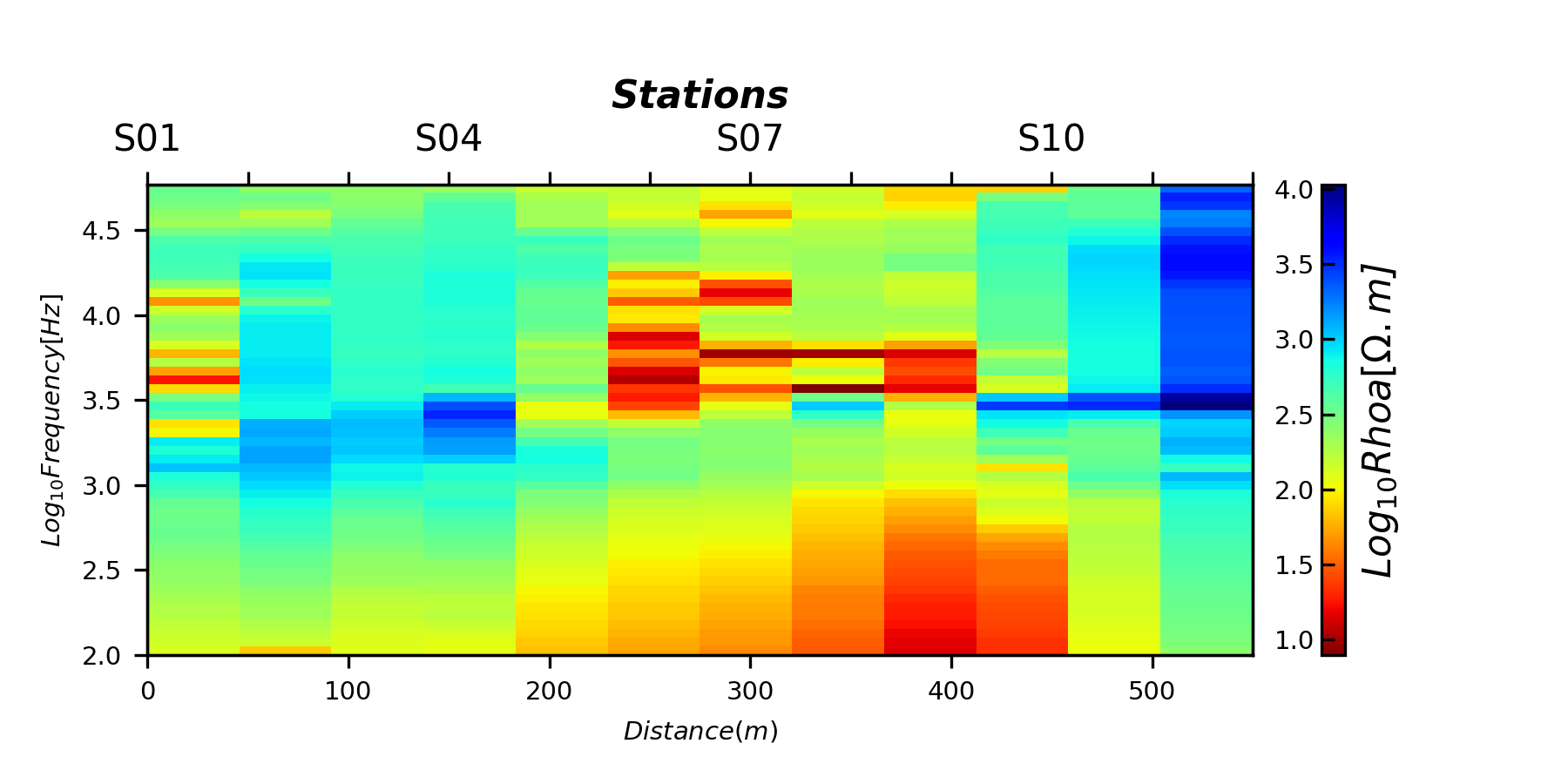
Plot two dimensional resistivity tensors

gives a quick visualization of resistivity tensors at the component ‘yx’ in a two-dimensional.

# Author: L.Kouadio
# Licence: BSD-3-clause

from watex.view.plot import TPlot
from watex.datasets import load_edis
# get some 3 samples of EDI for demo
edi_data = load_edis (return_data =True, samples =12)
# customize plot by adding plot_kws
plot_kws = dict( ylabel = '$Log_{10}Frequency [Hz]$',
                                            xlabel = '$Distance(m)$',
                                            cb_label = '$Log_{10}Rhoa[\Omega.m$]',
                                            fig_size =(6, 3),
                                            font_size =7.,
                                            plt_style ='imshow',
                                            )
t= TPlot(component='yx', **plot_kws).fit(edi_data)
# plot recovery2d using the log10 resistivity
t.plot_tensor2d (to_log10=True)

<AxesSubplot:xlabel='$Distance(m)$', ylabel='$Log_{10}Frequency [Hz]$'>