k-prediction from MXS: step-by-step guide

Real-world examples to generate the mixture learning strategy (MXS) target \(y*\) for predicting the permeability coefficient \(k\) parameter from two boreholes.

# Author: L.Kouadio
# Licence: BSD-3-clause

Note that this is an example of two boreholes which results is quited less relevant compared to the tangible example implemented in the Hongliu coal mine with 11 boreholes data [1]_.

We start by importing the required modules

import pandas as pd
from watex.datasets import load_hlogs

Preprocess data

Make a unique dataset from two boreholes data collected in Hongliu coal mine :h502 and h2601 and reduce down dimensions if necessary

# * load `load_hlogs` to get explicitly the features names and target names
box = load_hlogs ()
# combine our test data
# data  = load_hlogs().frame + load_hlogs(key= 'h2601').frame
data = load_hlogs (key ='*').frame
X0, y0 = data [box.feature_names] , data [box.target_names ]
# make copies for safety
X, y = X0.copy() , y0.copy()
# let's visualize the features names and target names
print("feature_names:\n" , box.feature_names )
print("target names:\n", box.target_names )

feature_names:
 ['hole_id', 'depth_top', 'depth_bottom', 'strata_name', 'rock_name', 'layer_thickness', 'resistivity', 'gamma_gamma', 'natural_gamma', 'sp', 'short_distance_gamma', 'well_diameter']
target names:
 ['aquifer_group', 'pumping_level', 'aquifer_thickness', 'hole_depth_before_pumping', 'hole_depth_after_pumping', 'hole_depth_loss', 'depth_starting_pumping', 'pumping_depth_at_the_end', 'pumping_depth', 'section_aperture', 'k', 'kp', 'r', 'rp', 'remark']

Data contains some categorical values, we will drop the rock name, the hole_id and well diameter which are subjective data and not useful for prediction puposes and impute the remaining data using a bi-impute strategy

from watex.utils import naive_imputer
X.drop (columns = ['rock_name', 'hole_id', 'well_diameter'] , inplace =True )

# * Merge both depths into one to compose only a single depth column
X['depth'] = ( X.depth_bottom + X.depth_top )/2
X.drop (columns =['depth_top', 'depth_bottom'], inplace =True )
data_imputed = naive_imputer( X , strategy='mean', mode='bi-impute')

• Use PCA analysis to reduce the dimension to down the important features

to predict the naive aquifer group (NGA).

# Note that for PCA analysis, we can remove the only categorial features
# "strata_name" and scaled the remaining features as follows:

from watex.utils import to_numeric_dtypes
from watex.utils import naive_scaler

# pop_cat_features auto-drop the only categorial features
Xpca = to_numeric_dtypes (data_imputed , pop_cat_features= True,
                          reset_index=True, drop_index =True,
                          verbose =True)
#  Scale the data  by default
Xpca_scaled = naive_scaler( Xpca )
Xpca_scaled_columns = list( Xpca_scaled.columns )
# * Call the normal PCA and plot all components set to None

from watex.analysis import nPCA

No NaN column found.
Feature:     1. strata_name  has been dropped from the dataframe.

• Plot explained variance ratio

pca = nPCA (Xpca_scaled , return_X= False, view = True ) # return PCA object rather than the reduced X

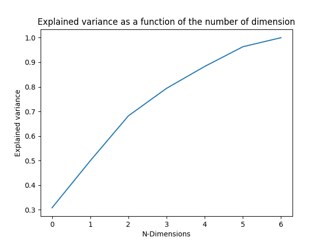
As a comment, here 5/6 features are enough since the explained variance ratio is already got 98 % * Set the number of components and use a convenient plot the both components

from watex.utils import plot_pca_components
pca = nPCA (Xpca_scaled ,n_components=2,  return_X=False ) # return object for plot purpose

components = pca.components_
features = pca.feature_names_in_
plot_pca_components (components, feature_names= features, cmap='jet_r')

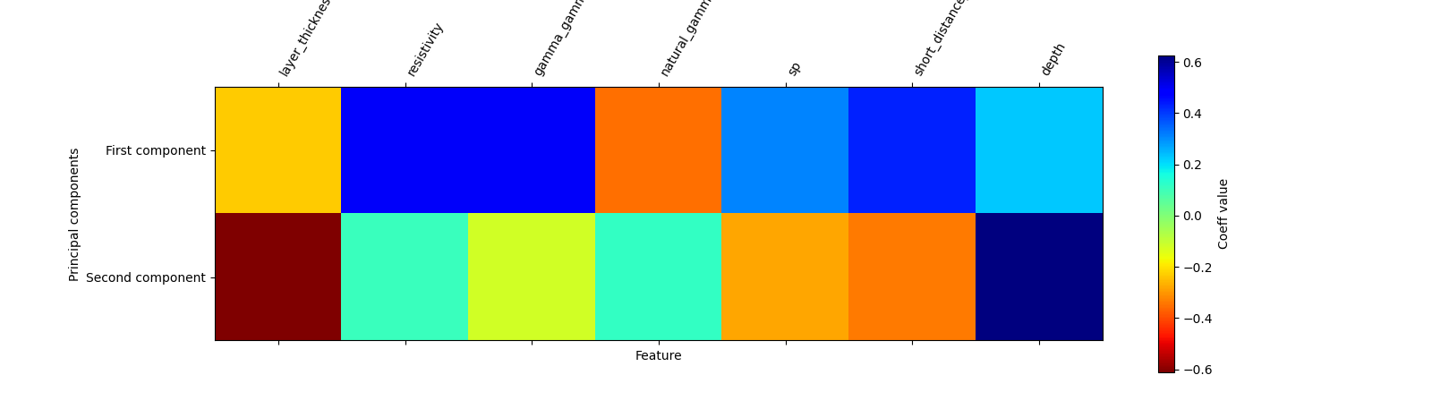
As comments, the matrix plot shows the contributions of all features in the first and second components. Indeed, while most contributions are got in-depth resistivity gamma and gamma short distance they are negatively correlated with layer thickness and natural gamma. However, no-correlation is found with the sp log data In the second components, the depth and natural gamma are more corollated and inversely correlated with the resistivity gamma, sp, and short distance. whereas the quasi-null correlation exists with layer thickness. By summarizing the PC1 and PC2 analysis, all features are useful as prediction and one of them can be skipped. This validates the explained variance ratio where under 8 features, after 7 dimensions, the explained variance ratio is already reached 98 %. Therefore features skipped should not influence the result of prediction

• Auto-preprocess the data using the default pipe

Note that the categorical data “strata_name” is one-hot-encoded and generate a sparse matrix ready for the data for prediction, then we will use the function ‘make_naive_pipe’ to fast encode and transform the data as output.

from watex.utils  import make_naive_pipe

# auto scaled the data and store it into a compressed sparse matrix format
csr_data = make_naive_pipe(data_imputed, transform= True) # auto-scaled the data using StandardScaler and  transform the data in place
csr_data

<1148x24 sparse matrix of type '<class 'numpy.float64'>'
    with 9158 stored elements in Compressed Sparse Row format>

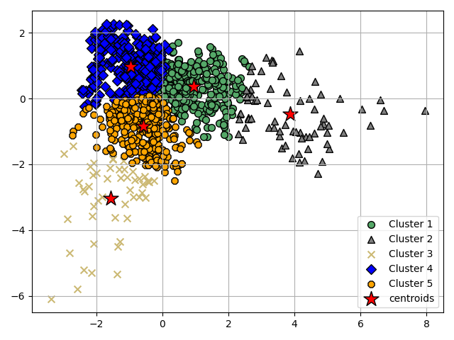
Prediction of Naive Group of Aquifer (NGA)

We randomly set the number of clusters to 05 which might correspond to the number of aquifer groups in the survey area according to the geological information. KMeans is used to predict the class label instead and plot the clusters

from watex.exlib.sklearn import KMeans
from watex.utils import plot_clusters

• Group the principal two components of PCA into the 5 clusters

km = KMeans (n_clusters =5 , init= 'random' )
ykm = km.fit_predict(pca.X  )
km3c = KMeans (n_clusters =3 , init= 'random' )
ykm3 = km3c.fit_predict(pca.X  )
# plot clusters into the general information of 5 groups of aquifers
plot_clusters (5 , pca.X, ykm , km.cluster_centers_ )

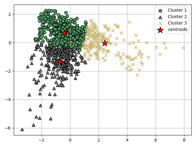
• Plot the 03 clusters

Now test the sample lot with only 03 clusters as a theory group of aquifer based on the distribution of the data.

plot_clusters (3 , pca.X, ykm3 , km3c.cluster_centers_ )

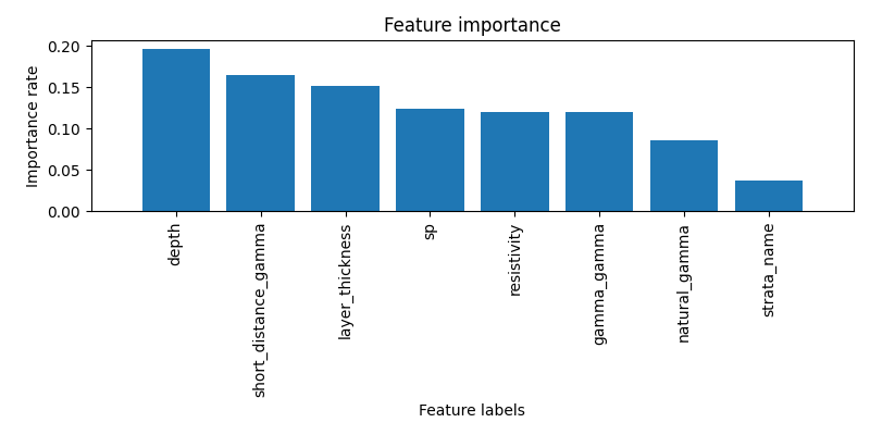
• Plot the feature’s importance

We encode the strata_name and add it to the scale value and plot_the feature importance

from watex.exlib.sklearn import RandomForestClassifier
from watex.utils import plot_rf_feature_importances

# add the strata_name to the remaining features
strata_column =  pd.Series ( X ['strata_name'].astype ('category').cat.codes , name ='strata_name' )
strata_column.index = range (len(strata_column))  # reindexing

X_for_fi = pd.concat( [ strata_column , Xpca_scaled ], axis =1, ignore_index=True )
# # plot importance with the predicted label ykm
X_for_fi=pd.DataFrame ( X_for_fi.values, columns= ['strata_name'] + Xpca_scaled_columns)
plot_rf_feature_importances (RandomForestClassifier(), X_for_fi , y =ykm )

plot elbow to confirm or infirm the 05 clustering of aquifers from geological infos

from watex.utils import plot_elbow
plot_elbow(pca.X, n_clusters=11)

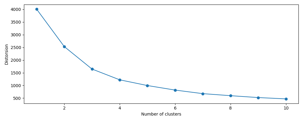
<AxesSubplot:xlabel='Number of clusters', ylabel='Distorsion'>

As comments, we can see, the elbow is located at k=3 that i.e we can classify the aquifer group based on the current datasets into three groups in hongliu coal mine. Note that the dataset is only for boreholes, this can not confirm the exact number of the aquifer. In the case study data applied in Honliu coal mine composed of 11 boreholes, the number of 03 clusters is selected although the 05 clusters do not indicate a bad clustering after a silhouette plot. The number of 03 is finally ascertained using the Hierarchical Agglomerative clustering (HAC) dendrogram plot. The step are enumerated below:

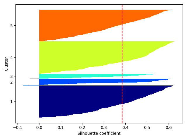
Let’s confirm the 05 clusters using the silhouette plot from KMeans

from watex.view import plotSilhouette
# plot silhouette for the 05 clusters with pca reduced data
plotSilhouette (pca.X, labels =ykm , prefit =True)

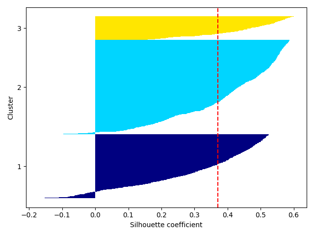
Plot with the 03 custers; plot silhouette for the three clusters by setting prefit to False since a new prediction should be made under the hood after n-iterations to find the best clustering. Refer to plotSilhouette() documentation.

plotSilhouette (pca.X, n_clusters= 3 , prefit =False)

Finally, we plot the dendrogram from HAC

from watex.view import plotDendrogram
plotDendrogram (pca.X , labels = ykm)

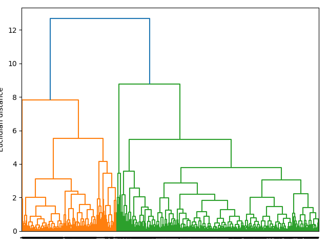
As comments in the case of MXS target, merging the predicted y with cluster =5 with create a lot of y=k33’ where we expected to have a list a =balance target with the true labels y (k1, k2 and k3 ) therefore the cluster with 3 labels is used instead of 5 thus the predicted NGA labels with true labels is combined with the the true labels y for supervised learnings. Note that the true labels are not altered by the predicted label y not let plot the dendro-heat

Before predicting the NGA labels, we can fit the aquifer group and find the most representative of the true k labels to the predicted labels test with the number of clusters set to 3

from watex.utils.hydroutils import find_aquifer_groups, classify_k
# categorize the k-values using the default func
yk_map =classify_k (y.k , default_func =True)
groupobj = find_aquifer_groups (yk_map,  ykm )
print(groupobj)
# now make the prediction
from watex.utils import predict_NGA_labels

yNGA = predict_NGA_labels(pca.X, n_clusters= 3)

_Group(Label=[' 1 ',
                   Preponderance( rate = '53.141  %',
                                [('Groups', {5: 0.468, 1: 0.236, 4: 0.217, 2: 0.049, 3: 0.03}),
                                 ('Representativity', ( '5', 0.47)),
                                 ('Similarity', '5')])],
             Label=[' 2 ',
                   Preponderance( rate = ' 19.11  %',
                                [('Groups', {5: 0.452, 1: 0.301, 4: 0.123, 2: 0.11, 3: 0.014}),
                                 ('Representativity', ( '5', 0.45)),
                                 ('Similarity', '5')])],
             Label=[' 3 ',
                   Preponderance( rate = '27.749  %',
                                [('Groups', {4: 0.491, 1: 0.443, 5: 0.038, 2: 0.028}),
                                 ('Representativity', ( '4', 0.49)),
                                 ('Similarity', '4')])],
             )

Prediction of MXS target \(y*\)

The prediction of MXS can simply be made by calling the function make_MXS_labels() or use the MXS class (MXS ) of the module hydro

from watex.utils import make_MXS_labels

yMXS = make_MXS_labels(y_true=yk_map , y_pred=yNGA )
# Let’s print the 12 firstMXS target
print(yMXS[:12])

['2*' '2*' '2*' '2*' '2*' '2*' '2*' '2*' '2*' '2*' '2*' '2*']

As a comment, the existing \(21\) and math:2* in the \(y*(yMXS)\) indicates that there is a strong similarity found between label 2 in the permeability coefficient dataset \(y\) and the predicted yNGA labels. This is validated by the group preponderance object above. Whilst, the math:2* indicates that the label 2 in yNGA has no similarity found in \(y*(yMXS)\)). The label 3 in yNGA has no relationship with any labels in the \(y\) therefore no modification is occurred and kept safe. If the parameter return_obj is set to True, it will return an MXS object where many attributes like class mapping can be retrieved for understanding purposes. for instance:

mxso = make_MXS_labels(y_true=yk_map , y_pred=yNGA , return_obj=True )
# similar labels
print(mxso.mxs_similarity_)

# group classes for mapping
print(mxso.mxs_group_classes_)

#M XS class mapping. This is usefull to know the labels that have been
# modified based on the similarity computation.
print(mxso.mxs_classes_)

# Once the :math:`y*(yMXS)` is predicted, the supervised learning model
# training can be made with the predictor:math:`X`.

[11, 21, 31]
{1: 11, 2: '2*', 3: '3*'}
['1' '11' '2' '2*' '3' '3*']

A paper is under puclication in Engineering Geology for k-prediction which explained a concrete study (Case study in Hongliu coal mine). See the reference in the citation page.