NSAMT tensors recovery

Recovers NSAMT tensors from sample of EDI files.

# Author: L.Kouadio
# Licence: BSD-3-clause

Tensor recovery is necessary when dealing with NSAMT data. The code below is an example to recover the weak and missing frequency signal using .em processing methods. The tensor recovery and the data quality control are ensured by the methods zrestore() and qc() respectively. The TPlot module from .view is used for the visualization. For a demonstration, I collect twelve samples of EDI objects stored in the software as:

from watex.datasets import load_edis
from watex.methods import EMAP
from watex.view import TPlot
edi_data = load_edis (return_data =True, samples =12 )
new_Z =EMAP().fit(edi_data ).zrestore ()

The method exportedis() can be used to export the new tensor (new_Z) ready for modeling. In the example below (umcommented), I use raw non-preprocessed EDI data as raw_data that includes missing tensor and weak frequency signals. The complete case data history data can be available upon request. Thus the recovered resistivity tensor from randomly sites E12 and E27 can be visualized by feeding the “raw_data” to the fit method of TPlot as follow:

# >>> TPlot().fit(<<raw_data>>).plot_multiple_recovery (sites =['E12', 'E27'])

Refer to EM method for the output

After recovering the signal, the latter exhibits a field strength amplitude for the next processing step like filtering. A simple filtering like adaptative moving average (AMA) proposed by Torres-verdìn and Bostick, (1992) can be used by simply calling:

edi_corrected =EMAP (window_size =5, c =2 ).fit(edi_data ).ama ()
# where 'c' is a window-width expansion factor inputted to the filter adaptation process to control
# the roll-off characteristics of the Hanning window (Torres-verdìn and Bostick, 1992).

Note that, like all the view plotting classes, TPlot inherits from a global abstract base class parameters BasePlot. Thus, each plot can flexibly be customized according to the user’s desire. For instance, to visualize the corrected 2D tensors, one can customize its plot as:

plot_kws = dict(
ylabel = '$Log_{10}Frequency [Hz]$',
xlabel = '$Distance(m)$',
cb_label = '$Log_{10}Rhoa[\Omega.m]$',
fig_size =(6, 3),
font_size =7)

Let visualize the raw-tensor and compared to the filtered tensors

TPlot(**plot_kws).fit(edi_data).plot_tensor2d(to_log10 =True)

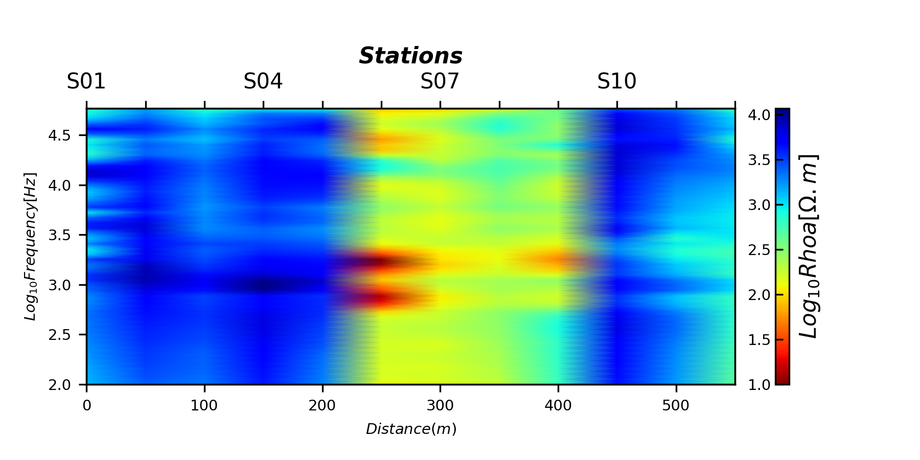
<AxesSubplot:xlabel='$Distance(m)$', ylabel='$Log_{10}Frequency [Hz]$'>

Let visualize the filtered tensors pass to parameter ffilter:

• Triming moving average (TMA) ( tma is the default filter)

TPlot(**plot_kws ).fit(edi_data). plot_ctensor2d (to_log10=True)

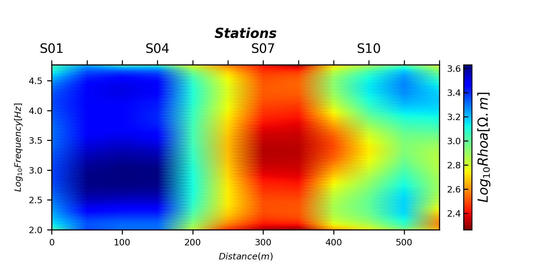
<AxesSubplot:xlabel='$Distance(m)$', ylabel='$Log_{10}Frequency [Hz]$'>

• Fixed-length-dipole (FLMA)

TPlot(**plot_kws ).fit(edi_data).plot_ctensor2d(to_log10 =True, ffilter ='flma')

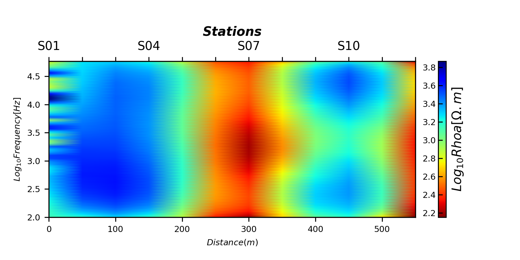
<AxesSubplot:xlabel='$Distance(m)$', ylabel='$Log_{10}Frequency [Hz]$'>

• Fixed-length-dipole (FLMA)

TPlot(**plot_kws ).fit(edi_data).plot_ctensor2d(to_log10 =True, ffilter ='ama')

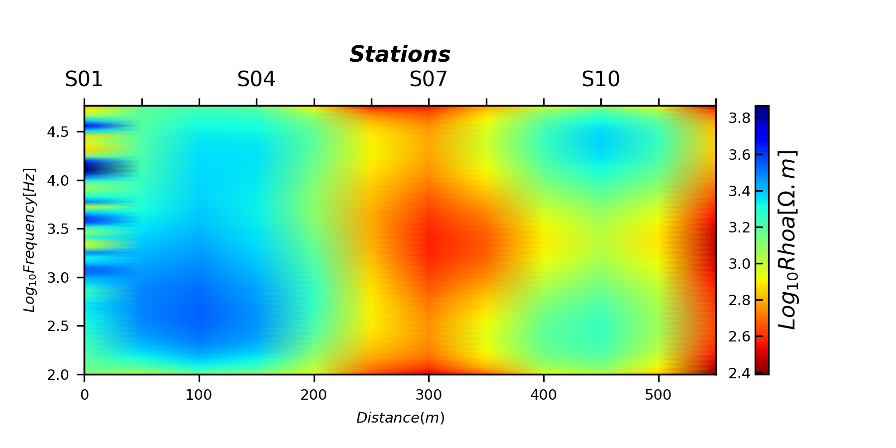
<AxesSubplot:xlabel='$Distance(m)$', ylabel='$Log_{10}Frequency [Hz]$'>