Note
Go to the end to download the full example code or to run this example in your browser via Binder
Predict FR from DC-Resistivity data#
shows some steps for predicting flow rate(FR) from DC-ERP and VES data
# Author: L.Kouadio
# Licence: BSD-3-clause
Import the required modules
from watex.datasets import fetch_data
from watex.datasets import load_gbalo, load_tankesse, load_bagoue
from watex.methods import ResistivityProfiling, VerticalSounding
from watex.methods import DCProfiling, DCSounding
from watex.view.plot import QuickPlot
from watex.models import pModels
from watex.exlib import train_test_split, accuracy_score
The raw DC data is recorded in zenodo during the drinking water supply campaign (DWSC) in 2012-2014 in Cote d’Ivoire in partnership with global organizations. The objective was to supply 2000 villages with potable water. The geophysical companies were associated with drilling ventures to locate the best position to carry out the drilling operations. The data is free of charge and can be distributed to a third party provided that it cites the authors as a reference. First, I randomly fetch the raw DC profiling and sounding data of one of these localities (Gbalo) during the DWSC project as:
gdata= load_gbalo ()
gdata.head(2)
Secondly, I will compute the DC prediction parameters by calling the
appropriate methods. For demonstration, I assume that the drilling is
performed at station 5(S05) on the survey line, i.e the DC parameters are
computed at that station. However, if the station is not specified,
the algorithm will find the best conductive zone based on the resistivity
values and will store the value in attribute sves_ (position to locate a drill).
The auto-detection can be used when users need to propose a place to make a
drill. Note that for a real case study, it is recommended to specify the
station where the drilling operation was performed through the parameter
station. For instance, automatic drilling location detection can predict a
station located in a marsh area that is not a suitable place for making a
drill. Therefore, to avoid any misinterpretation due to the complexity of
the geological area, it is useful to provide the station position. The
code snippets are:
erpo = ResistivityProfiling (station = 'S05').fit(gdata )
erpo.conductive_zone_  #(1)
array([1345, 1369, 1406, 1543, 1480, 1517, 1754])
erpo.summary(keep_params=True,return_table= True) #(2)
#(1) shows the resistivity of the best conductive zone and #(2) returns
the main prediction parameters. For reading multiple ERP data, it is
suggested to use the DCProfiling method. It performs
the same task but each parameter is stored in a line object. Let’s go ahead
by fetching another locality of ERP data (Tankesse) for demonstration:
dcpo= DCProfiling (stations =['S05', 'S07'] ).fit(gdata, load_tankesse() )
dcpo.nlines_ #(3)
dc-erp  :   0%|                                         | 0/2 [00:00<?, ?B/s]
dc-erp  : 100%|################################| 2/2 [00:00<00:00, 177.11B/s]

2
dcpo.line1.conductive_zone_ #(4)
array([1345, 1369, 1406, 1543, 1480, 1517, 1754])
dcpo.line1.sfi_
array([0.92600271])
#(3) shows the number of the given lines (line 1 for ERP Gbalo and
line 2 for ERP Tankesse. The line 1 value in #(4) computed from
multiple DC-profiling is similar to the individual computation of the
same line in (1) although the first approach gives multiple other features
such as the conductive zone visualization with the plotAnomaly method/function.
The same scheme for sounding parameter computation can be done with
the VerticalSounding and DCSounding.
Note that the latter saves data into a site object and not in line. For instance:
gvdata= load_gbalo (kind ='ves')
veso= VerticalSounding (search= 45 ).fit(gvdata)
dcvo = DCSounding(search=45).fit(gvdata)
veso.ohmic_area_
dc-ves  :   0%|                                         | 0/1 [00:00<?, ?B/s]
dc-ves  : 100%|################################| 1/1 [00:00<00:00, 149.47B/s]

268.0877145032066
dcvo.site1.ohmic_area_
268.0877145032066
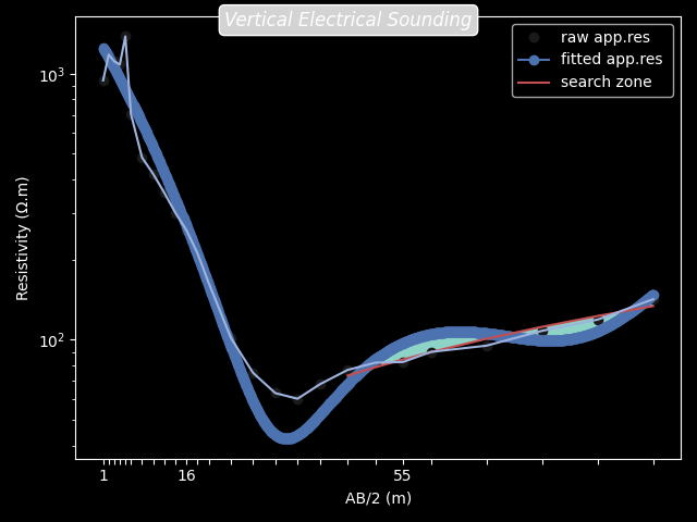
The search parameter passed to the above class is useful to find water
outside of the pollution. Usually, when the VES is performed, we are
expecting groundwater in the fractured rock in deeper that is outside of
any anthropic pollution (Biemi, 1992). Thus, the search parameter indicates
where the search of the fracture zone in deeper must start. For instance,
search=45 tells the algorithm to start detecting the fracture zone from 45m
to deeper (Figure below). In addition, when computing the prediction parameter
like ohmic-area (ohmS) of multiple sounding data for prediction purposes,
it is strongly recommended to settle the search argument unchangeable
for all sounding sites.
veso.plotOhmicArea(fbtw=True , style ='dark_background')
Furthermore, the DC parameters from the summary()
methods are combined with the geological data of the survey area to
compose the predictor \(X\). One of the interesting features of computing the
DC parameters for prediction purposes is to discuss the features.
This is possible with the discussingfeatures()
method of QuickPlot. An example of code snippets for
discussing plot is given below using the complete Bagoue DC parameters
computed from 431 boreholes:
.. GENERATED FROM PYTHON SOURCE LINES 116-131
data = load_bagoue ().frame
qkObj = QuickPlot( leg_kws={'loc':'upper right'},
fig_title = '`sfi` vs`ohmS|`geol`',
)
qkObj.tname='flow' # target the DC-flow rate prediction dataset
qkObj.mapflow=True # to hold category FR0, FR1 etc..
qkObj.fit(data)
sns_pkws={'aspect':2 ,
"height": 2,
}
map_kws={'edgecolor':"w"}
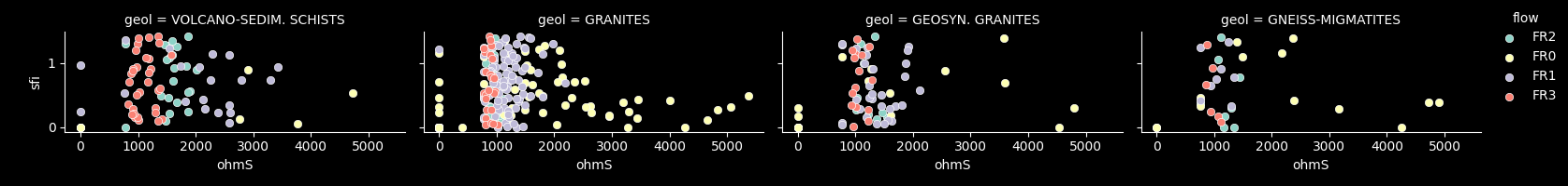
qkObj.discussingfeatures(features =['ohmS', 'sfi','geol', 'flow'],
map_kws=map_kws, **sns_pkws
)
QuickPlot(savefig= None, fig_num= 1, fig_size= (12, 8), ... , classes= None, tname= flow, mapflow= True)
As a comment of discussing features above. Figure shows at a glance
that most of the drillings carried out on granites have an FR of around
\(1 m^3/hr\) (FR1: 0< FR <=1). With these kinds of
flows, it is obvious that the boreholes will be unproductive (unsustainable)
within a few years. However, the volcano-sedimentary schists seem the most
suitable geological structure with an FR greater than \(3m^3/hr\).
However, the wide fractures on these formations (explained by ohmS > 1500)
do not mean that they should be more productive since all of the drillings performed
on the wide fracture do not always give a productive FR ( \(FR>3m^3/hr\))
contrary to the narrow fractures (around 1000 ohmS). As a result, it is reliable to
consider this approach during a future DWSC such as the geology of the area
and also the rock fracturing ratio computed thanks to the parameters
sfi and ohmS.
The following examples demonstrate how to predict FR with a complete
preprocessed dataset of DC parameters. The pre-trained models (optimal
model with acceptable variance and bias) of pModels
can be used to predict FR as:
X, y = fetch_data ('bagoue prepared data')
X_train, X_test, y_train, y_test = train_test_split (
    X, y, test_size =0.2 )
pmo = pModels (model='svm', kernel ='poly').fit (X_train, y_train )
y_pred =  pmo.predict (X_test )
accuracy_score (y_test, y_pred )
0.7246376811594203
Note the pre-trained estimator is stored in an attribute estimator_.
For instance, the pre-trained SVM model can be retrieved using
pmo.estimator_
or
pmo.SVM.poly.best_estimator_
If the model is not a kernel machine, the kernel attribute is discarded instead. For example:
pmo=pModels(model ='xgboost').fit (X_train, y_train )

# where xgboost stands for extreme gradient boosting machine(Friedman, 2001)
# and  the pre-trained estimator could be retrieved as
pmo.XGB.best_estimator_
Let make a new prediction with XGB
y_pred =  pmo.predict (X_test )
accuracy_score (y_test, y_pred )
0.8115942028985508
Total running time of the script: (0 minutes 1.588 seconds)