Plot pseudo-fracturing index (sfi)

visualizes the pseudo-fracturing index (sfi) used to speculate about the apparent resistivity dispersion ratio around the cumulated sum of the resistivity values of the selected conductive zone.

# Author: L.Kouadio
# Licence: BSD-3-clause

Import required modules

import numpy as np
from watex.utils.exmath import sfi, plot_sfi
from watex.property import P

Compute the sfi values from generate resistivity values of of selected conductive zone.

rang = np.random.RandomState (42)
condzone = np.abs(rang.randn (7)) *1e2
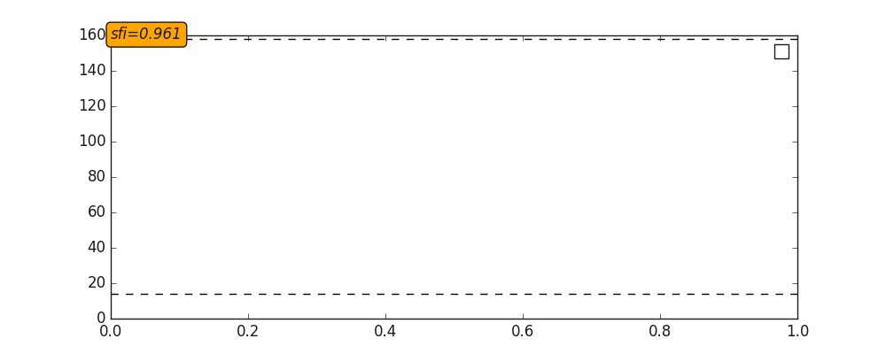
sfi_value = sfi (condzone)
print(sfi_value)

0.9606216039984983

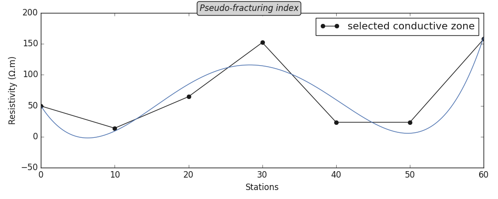
• Visualizes naive sfi with selected conductive zone.

Note

sfi has a view parameter to simply visualize the conductive zone.

The following code shows the naive visualization of the sfi to have quick depiction of the conductive zone.

plotkws  = dict (rlabel = 'Conductive zone (cz)',
                    label = 'fitting model',
                    leg =['selected conductive zone'],  # color=f'{P().frcolortags.get("fr3")}',
                    dtype='sfi',
                )
_= sfi (condzone, view= True , s= 5, fig_size = (10, 4), style ='classic',
          **plotkws )

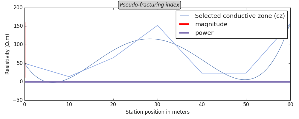
• Plot deep visualization with sfi components using plot_sfi()

plotkws  = dict (rlabel = 'Selected conductive zone (cz)',
                     #label = 'sfi fit-model',
                     color=f'{P().frcolortags.get("fr3")}',
                     )
plot_sfi (condzone,  fig_size = (10, 4), style ='classic', **plotkws)

• 
•