Note
Go to the end to download the full example code or to run this example in your browser via Binder
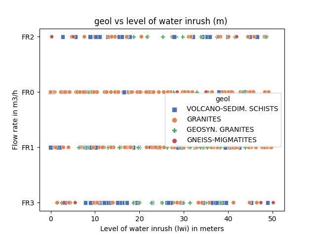
Plot scattering features#
visualizes correlation of two or more features with bivariate and univariate graphs.
# Author: L.Kouadio
# Licence: BSD-3-clause
from watex.view.plot import QuickPlot
from watex.datasets import load_bagoue
data = load_bagoue ().frame
qkObj = QuickPlot(lc='b', sns_style ='darkgrid',
fig_title='geol vs level of water inrush (m) ',
xlabel='Level of water inrush (lwi) in meters',
ylabel='Flow rate in m3/h'
)
qkObj.tname='flow' # target the DC-flow rate prediction dataset
qkObj.mapflow=True # to hold category FR0, FR1 etc..
qkObj.fig_size=(7, 5)
qkObj.fit(data)
marker_list= ['o','s','P', 'H']
markers_dict = {key:mv for key, mv in zip( list (
dict(qkObj.data ['geol'].value_counts(
normalize=True)).keys()),
marker_list)}
sns_pkws={'markers':markers_dict,
'sizes':(20, 200),
"hue":'geol',
'style':'geol',
"palette":'deep',
'legend':'full',
# "hue_norm":(0,7)
}
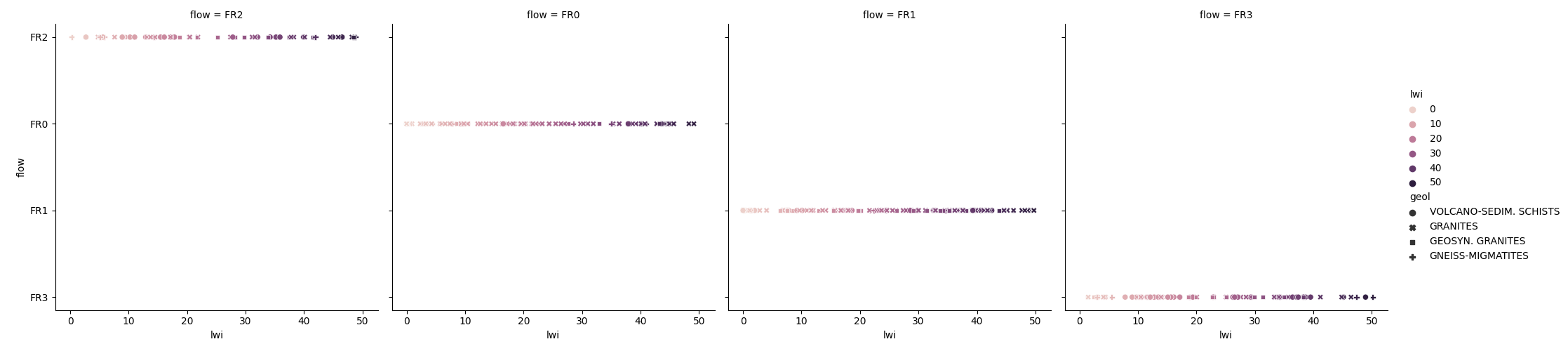
regpl_kws = {'col':'flow',
'hue':'lwi',
'style':'geol',
'kind':'scatter'
}
qkObj.scatteringfeatures(features=['lwi', 'flow'],
relplot_kws=regpl_kws,
**sns_pkws,
)
QuickPlot(savefig= None, fig_num= 1, fig_size= (7, 5), ... , classes= None, tname= flow, mapflow= True)
Total running time of the script: (0 minutes 1.712 seconds)