Plot electrical resistivity profiling (ERP)

shows the ERP and selected conductive zone.

# Author: L.Kouadio
# Licence: BSD-3-clause

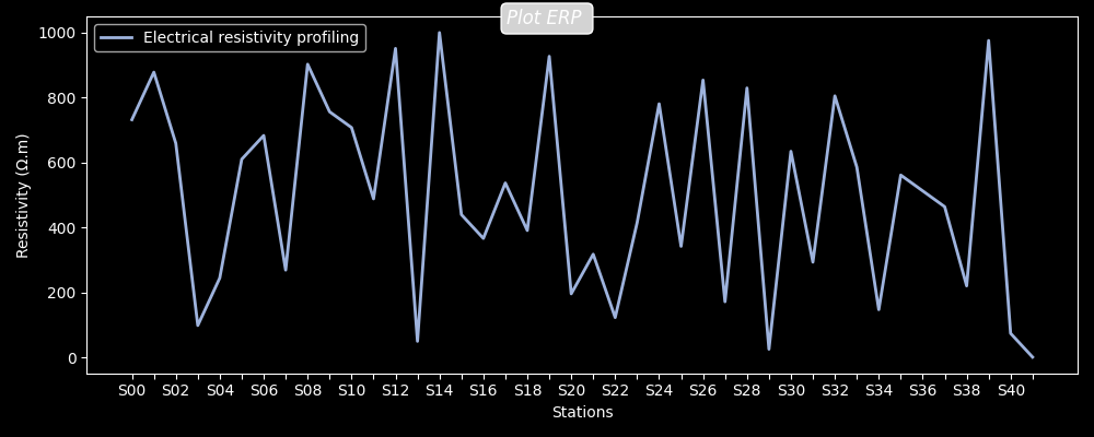
Generate synthetic data and plot the without any selected conductive zone. The synthetic ERP data can be generated using the function make_erp()

from watex.datasets import make_erp
from watex.utils.coreutils import plotAnomaly, defineConductiveZone
test_array = make_erp (stations = 30, seed = 0).frame.resistivity
# test_array = np.abs (np.random.randn (10) ) *1e2
plotAnomaly(test_array, style ="dark_background")

<AxesSubplot:xlabel='Stations', ylabel='Resistivity (Ω.m)'>

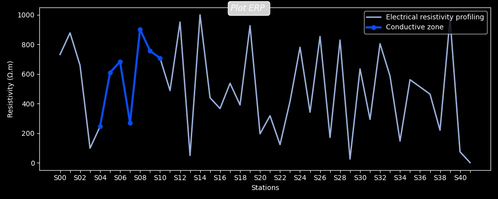
The conductive zone can be supplied mannualy as a subset of the erp or by specifying the station expected for drilling location.

selected_cz ,*_ = defineConductiveZone(test_array, station=7)
plotAnomaly(test_array, selected_cz , style ='dark_background')

<AxesSubplot:xlabel='Stations', ylabel='Resistivity (Ω.m)'>

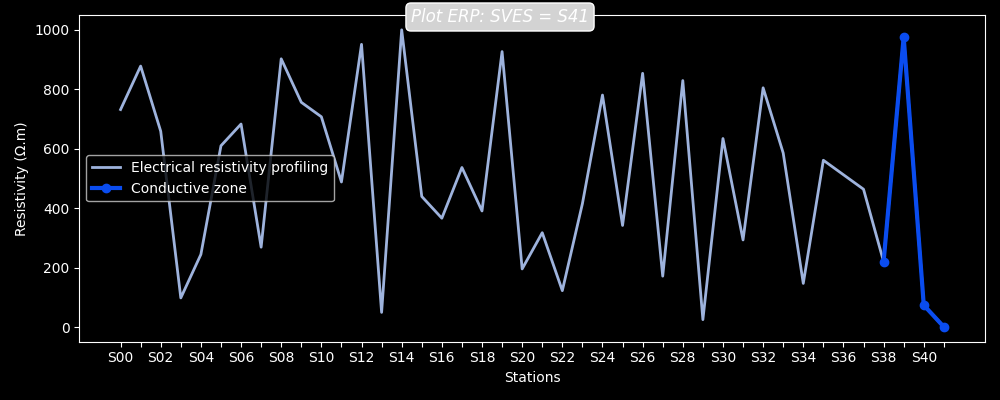
Automatic detect the position for making a drill by setting the station parameter to auto.

plotAnomaly(test_array, station= 'auto', style ='dark_background')

# Note
# ------
#   The auto-detection can be used when users need to propose a place to
#   make a drill.  Commonly for a real case study, it is recommended to
#   specify the station where the drilling operation was performed through
#   the parameter `station`. For instance, automatic drilling location detection
#   can predict a station located in a marsh area that is not a suitable place
#   for making a drill. Therefore, to avoid any misinterpretation due to the
#   complexity of the geological area, it is useful to provide the station
#   position.

<AxesSubplot:xlabel='Stations', ylabel='Resistivity (Ω.m)'>