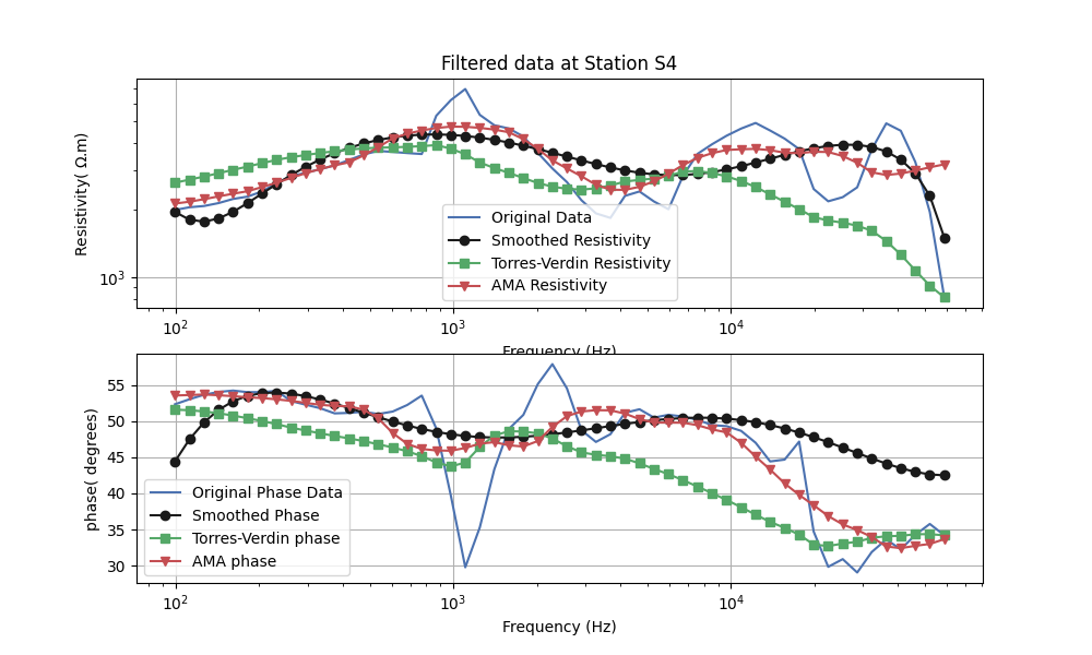
Remove noises

Filtered data to remove outliers, artifacts and existing noises in AMT data

# Author: L.Kouadio
# Licence: BSD-3-clause

Import required modules

import matplotlib.pyplot as plt
import watex as wx
from watex.methods.em import filter_noises

Fetch EDI data for the tests and load EM EDI objects using the Processing class. The demonstration will focus on the first station S00

edi_data = wx.fetch_data ('edis', samples =25 , return_data =True )
p= wx.EMAP ( ).fit(edi_data)

Print print seven values of resistivity and phase of the first station

station_index =4
print(p.ediObjs_[station_index].Z.resistivity[:, 0, 1][:7])  # resistivity
# phase
print(p.ediObjs_[station_index].Z.phase[:, 0, 1][:7]) #  phase
# Impedance values
print(p.ediObjs_[station_index].Z.z[:, 0, 1][:7])  # impedance tensor

[ 810.3093 1961.8073 3286.6644 4534.5832 4894.6956 3744.1404 2527.8144]
[34.1924 35.7665 34.2575 32.2367 33.6213 31.8762 29.0344]
[12766.91 +8673.923j 18348.04+13216.7j   22777.28+15512.85j
 25780.15+16257.67j  24827.42+16508.58j  20849.86+12965.86j
 16608.03 +9219.031j]

Compute resistivity and phase from filters * base smooth filter with method set to base ( default) * Torres-Verdin filter with method set to tv * Adaptive moving average filter with method set to ``ama`

res_b, phase_b = filter_noises (
    p, component='xy', return_z= False, )
res_t, phase_t = filter_noises (
    p, component='xy', return_z= False, method ='torres')
res_a, phase_a = filter_noises (
    p, component='xy', return_z= False, method ='ama')

Plot filtered data at station S00

fig, ax = plt.subplots(2,1, figsize =(10, 6))
ax[0].plot(p.freqs_, p.ediObjs_[station_index].Z.resistivity[:, 0, 1],
               'b-', label='Original Data')
ax[0].plot(p.freqs_, res_b[:, station_index], '-ok',
               label='Smoothed Resistivity')
ax[0].plot(p.freqs_, res_t[:, station_index], '-sg',
               label='Torres-Verdin Resistivity')
ax[0].plot(p.freqs_, res_a[:, station_index], '-vr',
               label='AMA Resistivity ')
ax[0].set_xlabel('Frequency (Hz)')
ax[0].set_ylabel('Resistivity( $\Omega$.m)')
ax[0].set_title(f'Filtered data at Station S{station_index}')
ax[0].set_yscale ('log')
ax[0].set_xscale ('log')
ax[0].legend()
ax[0].grid(True)
ax[1].plot(p.freqs_, p.ediObjs_[station_index].Z.phase[:, 0, 1],
               'b-', label='Original Phase Data')
ax[1].plot(p.freqs_, phase_b[:, station_index], '-ok',
               label='Smoothed Phase')
ax[1].plot(p.freqs_, phase_t[:, station_index], '-sg',
               label='Torres-Verdin phase')
ax[1].plot(p.freqs_, phase_a[:, station_index], '-vr',
               label='AMA phase')
ax[1].set_xlabel('Frequency (Hz)')
ax[1].set_ylabel('phase( degrees)')
ax[1].set_xscale ('log')
ax[1].legend()
ax[1].grid(True)
plt.show()