Plot Sequential Backward Selection (SBS)

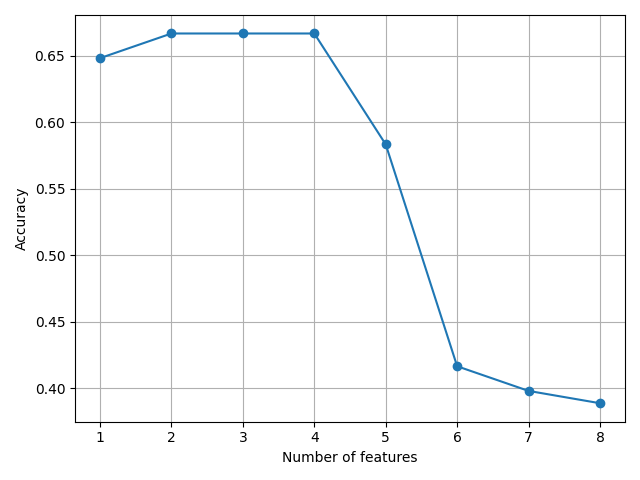
shows the SBS in action with the classification accuracy of the KNeighbors Classifier that was calculated on the validation dataset.

# Author: L.Kouadio
# Licence: BSD-3

imort the required modules and preprocess the data

from watex.datasets import fetch_data
from watex.exlib.sklearn import SimpleImputer
from watex.utils import selectfeatures
import matplotlib.pyplot as plt
from watex.exlib.sklearn import KNeighborsClassifier
from watex.base import SequentialBackwardSelection

data= fetch_data("bagoue original").get('data=dfy1') # encoded flow categories
y = data.flow ; X= data.drop(columns='flow')
# select the numerical features
X =selectfeatures(X, include ='number')
# imputed the missing data
X = SimpleImputer().fit_transform(X)

knn = KNeighborsClassifier(n_neighbors=5)
sbs= SequentialBackwardSelection(knn, k_features=1)
sbs.fit(X, y)

k_feat = [len(k) for k in sbs.subsets_]
plt.plot (k_feat, sbs.scores_, marker ='o')
#plt.ylim ([])
plt.ylabel ('Accuracy')
plt.xlabel ("Number of features")
plt.grid ()
plt.tight_layout()
plt.show()

# AS we can see the classifier achieve more than 70% accuracy for
# k =3, 4, 5. Thus, we can reduce the number of features down to.