K-Means Featurization

Featurize data for boosting the prediction and enforce the model to generalization

# License: BSD-3-clause
# Author: L.Kouadio

KMeans Featurisation ( KMF) is a surrogate booster to predict permeability coefficient (k) before any drilling construction. Indeed, KMF creates a compressed spatial index of the data which can be fed into the model for ease of learning and enforce the model capability of generalization. A new predictor based on model stacking technique is built with full target k which balances the spatial distribution of k-labels by clustering the original data.

We start by importing the required modules

import copy
import matplotlib.pyplot as plt
import scipy
import numpy as np

from sklearn.datasets import make_moons
from sklearn.linear_model import LogisticRegression
from sklearn.ensemble import GradientBoostingClassifier
from watex.datasets import load_mxs

from watex.transformers import featurize_X,  KMeansFeaturizer
from watex.exlib import train_test_split, XGBClassifier, roc_auc_score,roc_curve
from watex.utils import plot_voronoi, plot_roc_curves, replace_data

• Set the adjusted models XGBClassifiers and Gradient Boosting trees.

Classifiers are initialized with fined tuned values and fixed the seed to 0 for data reproducing.

seed = 0

xgb_cluster = XGBClassifier(max_depth =13 , n_estimators =50 ,
                            learning_rate = 0.09,  booster = 'gbtree')
classifier_names = ['LR','Fine-tuned Boosted Trees']
classifiers = [LogisticRegression(random_state=seed),
               GradientBoostingClassifier(
                n_estimators=10, learning_rate=1.0,max_depth=5)]

• Create helpers functions

Helper function for roc visualization

def roc_visualization (
    Xtrain,
    Xtest,
    Xtrain_cluster,
    Xtest_cluster,
    ytrain,
    ytest,
    use_default_xgb=False
    ):
    #
    #Fit the XGB  adjusted hyperparameters with KMF features
    # or use the default XGB
    global xgb_cluster
    if use_default_xgb:
        # take the default
        xgb_cluster = XGBClassifier ()

    xgb_cluster.fit(Xtrain_cluster, ytrain  )
    # * Plot ROC curve for demo
    for model in classifiers:
        model.fit(Xtrain, ytrain)
    _, ax = plt.subplots (1, 1, figsize = (7, 7) )
    fpr_cluster, tpr_cluster, auc_score = test_roc(xgb_cluster, Xtest_cluster, ytest)
    ax.plot(fpr_cluster, tpr_cluster, 'r-',
            label=f'XGB with KMF: AUC= {round(auc_score, 2)}')

    for i, model in enumerate(classifiers):
        fpr, tpr , auc_score = test_roc(model, Xtest, ytest)
        ax.plot(fpr, tpr, label=classifier_names[i] +
                f' AUC ={round(auc_score,2)}')

    ax.plot([0, 1], [0, 1], 'k--')
    ax.legend()

    return ax

 # Helper function to evaluate classifier performance using ROC
def test_roc(model, data, labels):
    if hasattr(model, "decision_function"):
        predictions = model.decision_function(data)
    else:
        predictions = model.predict_proba(data)[:,1]
    fpr, tpr, _ = roc_curve(labels, predictions)
    auc_score = roc_auc_score(labels, predictions)

    return fpr, tpr, auc_score

Use concrete log data for KMF implementation

In this test case for implementing the K-Featurization (KMF) surrogate booster we use the hongliu 11 borehole data for application. We will separate the data into 80% training and 20% testing . Note that the hyperparameter should be fixed to avoid the learning process. We used the LogisticRegression, and Gradient boosting as the model for testing. We also fixed the random scale for reproducing the same data.

X, y = load_mxs ( key ='scale', return_X_y= True, samples ="*" , seed = seed)

# When using the Windows with MKL, you can called the function :func:`watex.utils.replace_data`
# to avoid the KMeans memory leak. Then uncomment this section
# X, y = replace_data(X, y, n_times = 2 )

• make binary datasets

construct the binary data sets from the target mapping then splitting the data. {0: ‘1’, 1: ‘11*’, 2: ‘2’, 3: ‘2*’, 4: ‘3’, 5: ‘33*’}

y [y <=2]= 0 ; y [y >0 ]=1
training_data, test_data, training_labels, test_labels = train_test_split (
    X, y , test_size =.2 )

# * Call KMeansFeaturizer to featurize the data X
kmf_hint = KMeansFeaturizer(n_clusters=100, target_scale=1).fit(training_data,
training_labels)
kmf_no_hint = KMeansFeaturizer(n_clusters=100, target_scale=0).fit(training_data,
training_labels
)
# Use the k-means featurizer to generate cluster features
# and sparse_matrix
training_cluster_features = kmf_hint.transform(training_data)
test_cluster_features = kmf_hint.transform(test_data)

training_with_cluster = np.concatenate ((training_data, training_cluster_features),
                                        axis =1 )
training_with_cluster= scipy.sparse.csr_matrix (training_with_cluster )
test_with_cluster = np.concatenate ((test_data, test_cluster_features),
                                        axis =1 )
test_with_cluster= scipy.sparse.csr_matrix(test_with_cluster)

• Plot roc curves

roc_visualization(Xtrain= training_data,
                  Xtest= test_data,
                  Xtrain_cluster= training_with_cluster,
                  Xtest_cluster= test_with_cluster,
                  ytrain=training_labels,
                  ytest= test_labels,
                  )

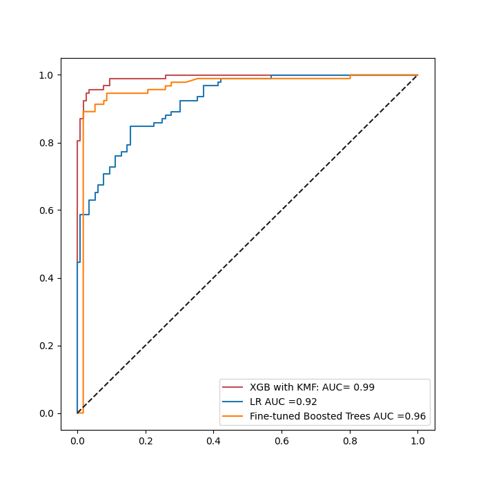
<AxesSubplot:>

Figure shows that the performace of fined_tuned XGB is greater than The fine-tuned XGB and LR without applying the KMFeatures.

• Plot separetly LR and BoostTrees with KMF

clfs = copy.deepcopy([classifiers[-1]])
clfs_cluster = [m.fit( training_with_cluster, training_labels) for m in clfs ]
ax = plot_roc_curves(clfs_cluster, test_with_cluster, test_labels, all=True, ncols = 2,
                fig_size = (10, 4), names = ['Boostree with KMF '],
                colors =['orange', 'r'], get_score =True )

for i, model in enumerate(clfs):
    model.fit(training_data, training_labels)
    fpr, tpr , auc_score = test_roc(model, test_data, test_labels)
    ax[1] .plot(fpr, tpr, label=classifier_names[-1] + f' AUC ={round(auc_score,2)}')
    ax[1].legend()

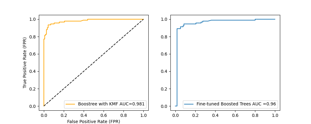
When comparing the GBoostree with KMF and without, there is a little bit improvement (+2.1%). This improvement should be more significant if the mixture learning strategy were not applied upstream into the Borehole data.

Use common Moon dataset

• Build models with a common data sets. (e.g. Moons dataset)

We generate 8000 samples of dataset where we divided as 50% training and 50% testing For reproducing the same samples of data, we fixed the seed. to reproduce the dataset

X0, y0= make_moons(n_samples =8000, noise= 0.2)
# make a test data
X0_test,  y0_test = make_moons(n_samples = 2000, noise= 0.3 )

• Voronoi plot 2D

Veronoi plot can be used to visualize the model using hint ( target associated) and without. For a human representation ( 2D), we used the most two features importances of the consistent data set.

fig, ax = plt.subplots(2,1, figsize =(7, 7))
kmf_hint = KMeansFeaturizer(n_clusters=200, target_scale=10).fit(X0,y0)
kmf_no_hint = KMeansFeaturizer(n_clusters=200, target_scale=0).fit(X0, y0)
plot_voronoi ( X0, y0 ,cluster_centers=kmf_hint.cluster_centers_,
                  fig_title ='KMF with hint', ax = ax [0] )
plot_voronoi ( X0, y0,cluster_centers=kmf_no_hint.cluster_centers_,
                  fig_title ='KMF No hint' , ax = ax[1])

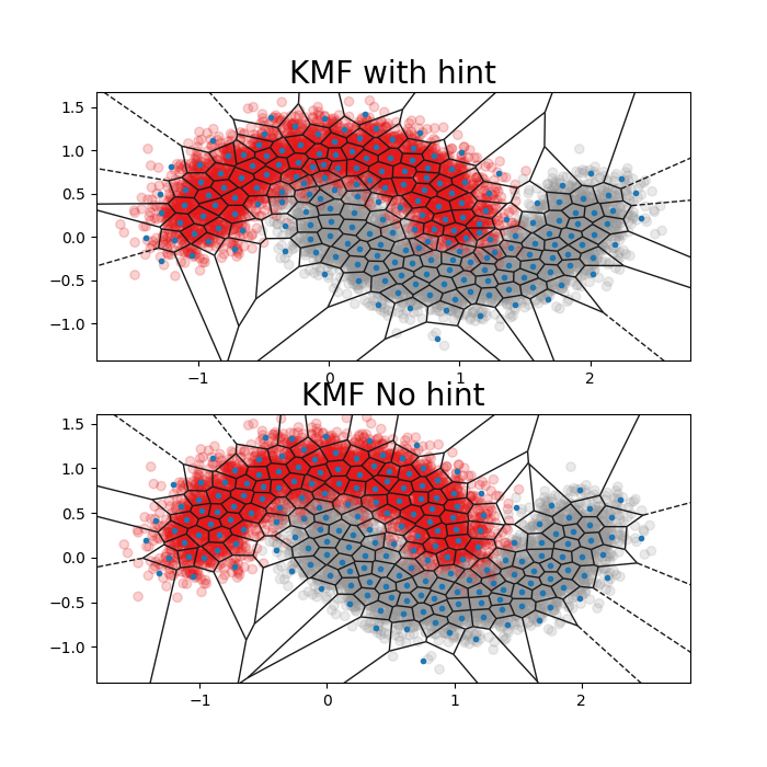
<AxesSubplot:title={'center':'KMF No hint'}>

The is a shortcut way to featurize data at once by calling the watex.transformers.featurize_X() to transform X data. It could also returns KMF_model if the parameter return_model is set to True.

X0_kmf_train, y0_kmf_train,  kmf_hint = featurize_X(
    X0, y0, n_clusters =100, target_scale =10, to_sparse =True,
    return_model =True , random_state=seed )

# featurize the test data separately
test_with_cluster, _ = featurize_X(X0_test, model =kmf_hint, to_sparse=True  )

As shown in the figure above. The number of clusters when target information is missed span too much of the space between the two classes. Commonly KMF demonstrates its usefulness when cluster boundaries align with class boundaries much more closely.

ax = roc_visualization (Xtrain= X0 ,
                   Xtest= X0_test ,
                   Xtrain_cluster= X0_kmf_train,
                   Xtest_cluster= test_with_cluster,
                   ytrain= y0,
                   ytest = y0_test,
                   use_default_xgb=True,
                   )

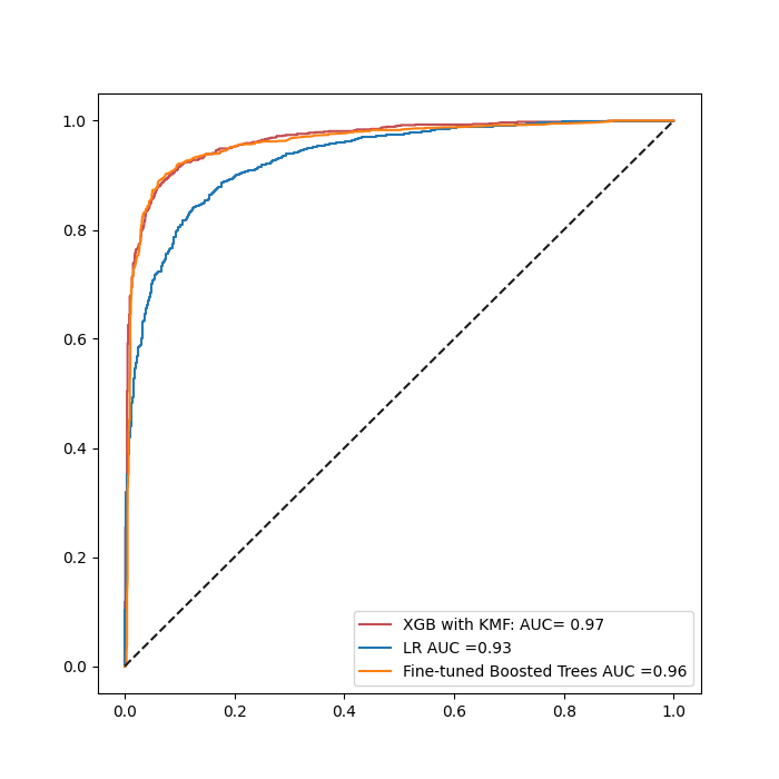
Conclusion

Based on both ROC curves, we can visualize KMF approach can work well on small data with a AUC=97% for XGB while the fine-tuned GB and LR have 96 % and 92 % respectively. When the data set becomes huge, XGB with KMF maintains its convergence score while other model preformances increases with the data. This is the case for Fine-tuned Gradient boosting ( 96%) and LR ( 93%). large amount of data ( e.g. Moon data sets ). The powerfull of KMF is its capability to well perform on a small dataset since it is the main challenge that it tries to solve especially in geosciences field where huge data is rare and owned by private companies.