EM, DC, and Hydro parameters computing

Real-world examples for showing the computation of EM tensor, DC parameters and how to implement the mixture learning strategy (MXS) from the naive aquifer group (NGA) for the permeability coefficient k prediction.

# Author: L.Kouadio
# Licence: BSD-3-clause

Import required modules

import numpy as np
import matplotlib.pyplot as plt
plt_style ='classic'

# Load real data collected during the drinking water supply campaign
# occured in 2012-2014 in Cote d'Ivoire. Read more in the dataset
# module ( :mod:`~watex.datasets`)
from watex.datasets import (
    load_edis,
    load_gbalo,
    load_semien,
    load_tankesse,
    load_boundiali
    )
# Real logging data collected in Hongliu coal mine, in China, Hunan province
from watex.datasets import load_hlogs
from watex.methods import(
    DCProfiling,
    DCSounding,
    ResistivityProfiling,
    VerticalSounding,Processing ,
    Logging,
    MXS
    )

EM em

The EM module is related to a few meter exploration in the case of groundwater exploration. The module provides some basic processing steps for EMAP data filtering and removing noises. Commonly the method mostly used in groundwater exploration is the audio-magnetotelluric because of the shortest frequency and rapid executions. Furthermore, we can also list some other advantages such as:

• is useful for imaging both deep geologic structure and near-surface geology and can provide significant details.

• includes a backpack portable system that allows for use in difficult terrain.

• the technique requires no high-voltage electrodes, and logistics are relatively easy to support in the field. Stations can be acquired almost anywhere and can be placed any distance apart. This allows for large-scale regional reconnaissance exploration or detailed surveys of local geology and has no environmental impact

note:

For deep implementation or exploring a large scale of EM/AMT data processing, it is recommended to use the package pycsamt. Create EM object as a collection of EDI-file. Collect edi-files and create an EM object. It sets he properties from audio-magnetotelluric. The two(2) components XY and YX will be set and calculated.Can read MT data instead, however, the full handling transfer function like Tipper and Spectra is not completed. Use other MT software for a long period’s data.

from watex.methods.em import EM
edi_data = load_edis (return_data =True, samples =7) # object from Edi_collection
emObjs = EM().fit(edi_data)
ref=emObjs.getfullfrequency ()
ref

emObjs.freqs_ # # however full frequency can just be fetched using the attribute `freqs_`

# get the reference frequency
rfreq = emObjs.getreferencefrequency ()
rfreq

# Fast process EMAP and AMT data. Tools are used for data sanitizing,
# removing noises and filtering.

p = Processing().fit(edi_data)
p.window_size =2
p.component ='yx'
rc= p.tma()
# get the resistivity value of the third frequency  at all stations
# >>> p.res2d_[3, :]

# get the resistivity value corrected at the third frequency
# >>> rc [3, :]

Plot 1D raw and corrected tensor

plt.semilogy (np.arange (p.res2d_.shape[1] ), p.res2d_[3, :], '--',
                  np.arange (p.res2d_.shape[1] ), rc[3, :], 'ok--')

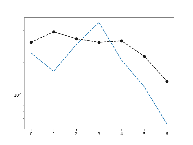
[<matplotlib.lines.Line2D object at 0x7fec8bd477c0>, <matplotlib.lines.Line2D object at 0x7fec8bd453c0>]

# Compute the skew: The conventional asymmetry parameter based on the Z magnitude.

# p = Processing().fit(edi_data)
# sk,_ = p.skew()
# sk[0:, ]

# restore tensor
pObjs= Processing().fit(edi_data)
# One can specify the frequency buffer like the example below, however
# it is not necessary at least there is a specific reason to fix the frequencies
# buffer = [1.45000e+04,1.11500e+01]
zobjs_b =  pObjs.zrestore(
    # buffer = buffer
)
zobjs_b

# control the quality of the EM data
#     pobj = Processing().fit(edi_data)
#     f = pobj.getfullfrequency ()
#     # len(f)
#     # ... 55 # 55 frequencies
#     c, = pobj.qc ( tol = .6 ) # mean 60% to consider the data as
#     # representatives
#     c  # the representative rate in the whole EDI- collection
#      # ... 0.95 # the whole data at all stations is safe to 95%.
#     # now check the interpolated frequency
#     c, freq_new,  = pobj.qc ( tol=.6 , return_freq =True)
#     # len(freq_new)
#     # ... 53  # delete two frequencies

array([<watex.externals.z.Z object at 0x7fec8faec400>,
       <watex.externals.z.Z object at 0x7fec8faefd00>,
       <watex.externals.z.Z object at 0x7fec8faef700>,
       <watex.externals.z.Z object at 0x7fec8b1f9630>,
       <watex.externals.z.Z object at 0x7fec8bdbf880>,
       <watex.externals.z.Z object at 0x7fec8faee320>,
       <watex.externals.z.Z object at 0x7fec8faefd30>], dtype=object)

DC-method electrical

A collection of DC-resistivity profiling and sounding classes. It reads and computes electrical parameters. Each line or site composes a specific object and gathers all the attributes of ResistivityProfiling or VerticalSounding for easy use. For instance, the expected drilling location point and its resistivity value for two survey lines ( line1 and line2) can be fetched

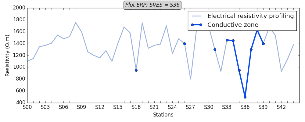
DC -Profiling

• Get DC -resistivity profiling from the individual Resistivity object

robj1= ResistivityProfiling(auto=True) # auto detection
robj1.utm_zone = '50N'
data = load_tankesse ()
robj1.fit(load_tankesse ())
print(robj1.sves_ )
robj2= ResistivityProfiling(auto=True, utm_zone='40S')
robj2.fit(load_gbalo())
print(robj2.sves_ )
# read the both objects
dcobjs = DCProfiling()
dcobjs.fit(robj1, robj2)
print(dcobjs.sves_ )

print(dcobjs.line1.sves_)
print(dcobjs.line2.sves_ )

S022
S036

dc-erp  :   0%|                                         | 0/2 [00:00<?, ?B/s]
dc-erp  : 100%|################################| 2/2 [00:00<00:00, 478.61B/s]
['S022' 'S036']
S022
S036

Plot conductive zone for line 1

robj1.plotAnomaly (style =plt_style)

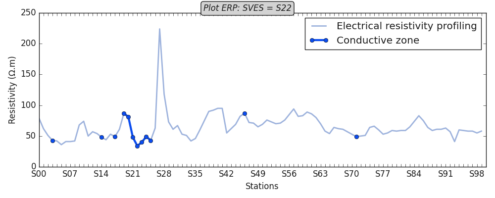
<AxesSubplot:xlabel='Stations', ylabel='Resistivity (Ω.m)'>

Plot conductive zones for second lines

robj2.plotAnomaly ( style = plt_style )

<AxesSubplot:xlabel='Stations', ylabel='Resistivity (Ω.m)'>

• Get parameters

robj1.summary(return_table=True )

	dipole	longitude	latitude	easting	northing	sves_resistivity	power	magnitude	shape	type	sfi
station
S022	10	109	-81	382775	896164	34	60	53	C	PC	0.31221

DC Sounding

• Read single sounding site

dsobj = DCSounding ()
dsobj.search = 30. # start detecting the fracture zone from 30m depth.
dsobj.fit(load_gbalo(kind ='ves'))
print(dsobj.ohmic_areas_)
print(dsobj.site1.fractured_zone_ )

dc-ves  :   0%|                                         | 0/1 [00:00<?, ?B/s]
dc-ves  : 100%|################################| 1/1 [00:00<00:00, 143.74B/s]
[569.03511708]
[ 28.  32.  36.  40.  45.  50.  55.  60.  70.  80.  90. 100.]

• read multiple sounding files

dsobj.search = 30 #[ 30, 30, 30, 30] # search values for all sites
dsobj.fit(load_semien(index_rhoa= 2 ),
          load_gbalo(kind ='ves', index_rhoa =2 ,),
          load_boundiali (index_rhoa=1)
          )
print(dsobj.ohmic_areas_ )
print(dsobj.nareas_ )

print(dsobj.survey_names_)

print(dsobj.nsites_ )

print(dsobj.site1.ohmic_area_)

print(dsobj.data_ )
# you can use the `isnotvalid_` attributes to check the unread data before
# calling the site object like
print("dsobj.isnotvalid_", dsobj.isnotvalid_) # return empty list if all values passed are correct.

dc-ves  :   0%|                                         | 0/3 [00:00<?, ?B/s]
dc-ves  : 100%|################################| 3/3 [00:00<00:00, 169.78B/s]
[ 572.84134545 1607.71498659  154.00420841]
[1. 2. 2.]
['site1' 'site2' 'site3']
3
572.8413454485877
[VerticalSounding(AB= 200.0, MN= 20.0, arrangememt= schlumberger, ... , h0= 1.0, strategy= HMCMC, xycoords= (nan, nan)), VerticalSounding(AB= 200.0, MN= 20.0, arrangememt= schlumberger, ... , h0= 1.0, strategy= HMCMC, xycoords= (nan, nan)), VerticalSounding(AB= 200.0, MN= 20.0, arrangememt= schlumberger, ... , h0= 1.0, strategy= HMCMC, xycoords= (nan, nan))]
dsobj.isnotvalid_ []

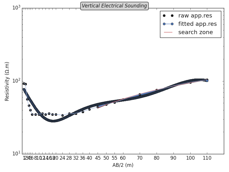
• Plot ohmic area

ves = VerticalSounding ().fit (dsobj.site3.data_)
ves.plotOhmicArea (fbtw=True , style =plt_style)

Hydrogeology hydro

Hydrogeological parameters of the aquifer are the essential and crucial basic data in the designing and construction progress of geotechnical engineering and groundwater dewatering, which is directly related to the reliability of these parameters.

# get the logging data
h = load_hlogs ()
print(h.feature_names)

['hole_id', 'depth_top', 'depth_bottom', 'strata_name', 'rock_name', 'layer_thickness', 'resistivity', 'gamma_gamma', 'natural_gamma', 'sp', 'short_distance_gamma', 'well_diameter']

we can collect the valid logging data and fit it

log= Logging(kname ='k', zname='depth_top' ).fit(h.frame[h.feature_names])
print( log.feature_names_in_)  # categorical features should be discarded.

['depth_top', 'depth_bottom', 'layer_thickness', 'resistivity', 'gamma_gamma', 'natural_gamma', 'sp', 'short_distance_gamma', 'well_diameter']

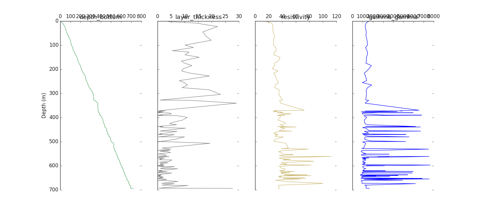
Plot default log using the predictor \(X\) ( composed of features only) As an example, we will plot the first five features

log= Logging(kname ='k', zname='depth_top' ).fit(h.frame[log.feature_names_in_[:5]])
log.plot ()

Logging(zname= depth_top, kname= k, verbose= 0)

Plot log including the target y

log.plot (y = h.frame.k , posiy =0 )# first position

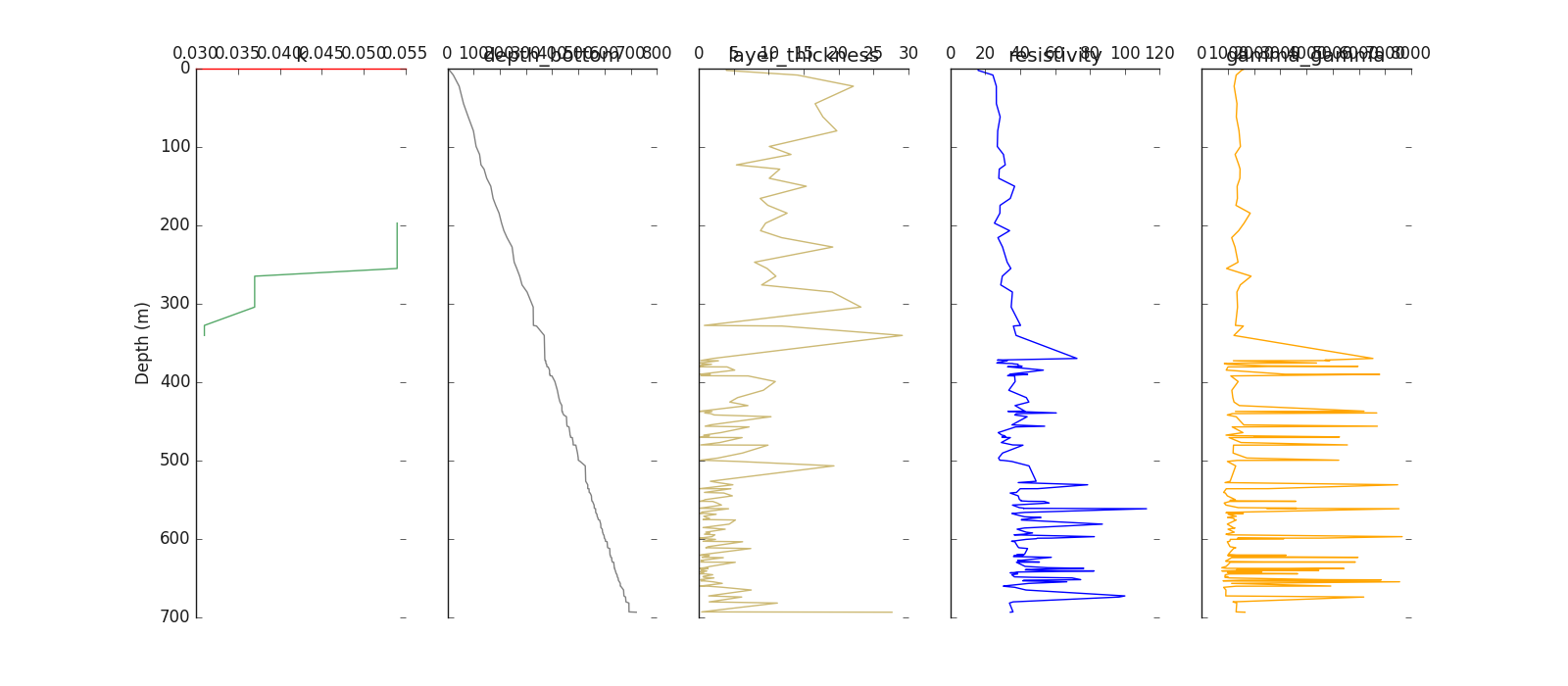
Logging(zname= depth_top, kname= k, verbose= 0)

Mixture Learning Strategy (MXS)

The use of machine learning for k-parameter prediction seems an alternative way to reduce the cost of data collection thereby saving money. However, the borehole data comes with a lot of missing k since the parameter is strongly tied to the aquifer after the pumping test. In other words, the k-parameter collection is feasible if the layer in the well is an aquifer. Unfortunately, predicting some samples of k in a large set of missing data remains an issue using the classical supervised learning methods. We, therefore, propose an alternative approach called a mixture of learning strategy (MXS) to solve these double issues. It entails predicting upstream a naïve group of aquifers (NGA) combined with the real values k to counterbalance the missing values and yield an optimal prediction score. The method, first, implies the K-Means and Hierarchical Agglomerative Clustering (HAC) algorithms. K-Means and HAC are used for NGA label predicting necessary for the MXS label merging.

hdata = load_hlogs ().frame
# drop the 'remark' columns since there is no valid data
hdata.drop (columns ='remark', inplace =True)
mxs = MXS (kname ='k').fit(hdata)
# predict the default NGA
mxs.predictNGA() # default prediction with n_groups =3
# make MXS labels using the default 'k' categorization
ymxs=mxs.makeyMXS(categorize_k=True, default_func=True)
print(mxs.yNGA_ [62:74] )

print(ymxs[62:74])
# array([ 1, 22, 22, 22,  3,  1, 22,  1, 22, 22,  1, 22])
# to get the label similarity , need to provide the
# the column name of the aquifer group and fit again like
mxs = MXS (kname ='k', aqname ='aquifer_group').fit(hdata)
sim = mxs.labelSimilarity()
print(sim )
# [(0, 'II')] # group II and label 0 are very similar

[1 2 2 2 3 1 2 1 2 2 1 2]
[ 1 22 22 22  3  1 22  1 22 22  1 22]
[(0, 'II')]

Once the MXS label is created, you can use the supervised training strategy for training models. Refer to the model modules (models)