Plot apparent resistivity curves

Plot station/site apparent resistivity curves

# Author: L.Kouadio
# Licence: BSD-3-clause

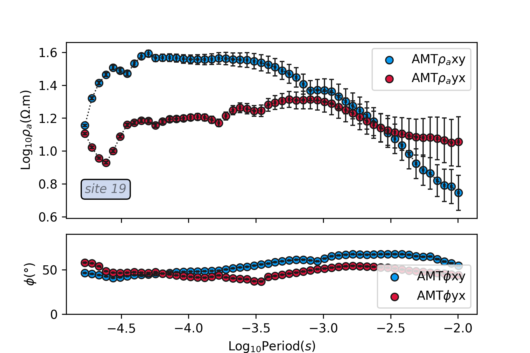
An example of plot apparent resistivity curves with error bar of EDI data collected in Huayaun province. seed is used to reproduce the data at the same station. * Simple Plot

import watex
test_data = watex.fetch_data ('huayuan', return_data =True , clear_cache=True )
tplot = watex.TPlot(fig_size =(6,  4), marker ='o').fit(test_data)
tplot.plt_style='classic'
tplot.plot_rhoa (seed =52, mode ='*', survey='AMT', show_site =True, )

<'TPlot':survey_area=None, distance=50.0, prefix='S', window_size=5, component='xy', mode='same', method='slinear', out='srho', how='py', c=2>

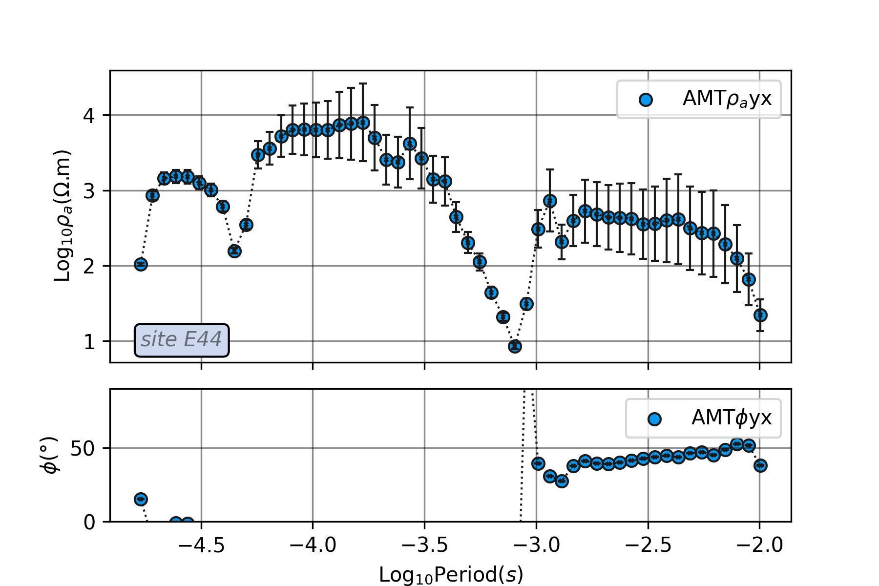
• Plot a specific EM data type

To plot a station data with no errorbar and a single component, we can set, errobar=False and specify the EM mode. For instance, we use the transverse electric mode TE for this example at station s44.

tplot.show_grid=True
tplot.plot_rhoa (site= 'E44', mode ='TM',survey='AMT', show_site =True ,
                seed = 52
                )

<'TPlot':survey_area=None, distance=50.0, prefix='S', window_size=5, component='xy', mode='same', method='slinear', out='srho', how='py', c=2>

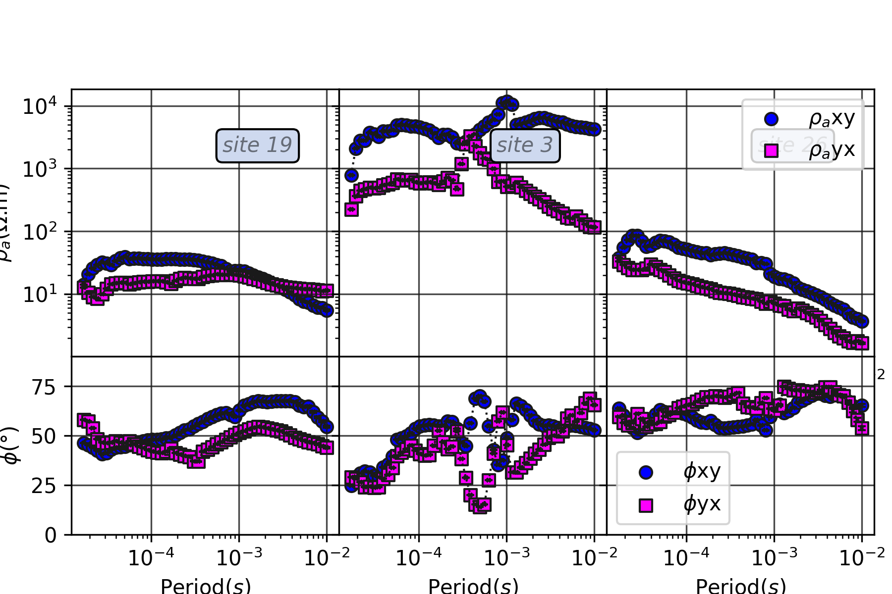
• Plot multiple sites

It is also possible to plot multiple stations. For instance, we can plot three sites using the watex.view.TPlot.plot_rhophi() by setting the parameters n_sites to 3 as:

tplot.gls =':' ; tplot.galpha=.8; tplot.gc ='k'
tplot.plot_rhophi ( n_sites = 3 , mode = '*', show_site =True, seed =52 )

<'TPlot':survey_area=None, distance=50.0, prefix='S', window_size=5, component='xy', mode='same', method='slinear', out='srho', how='py', c=2>

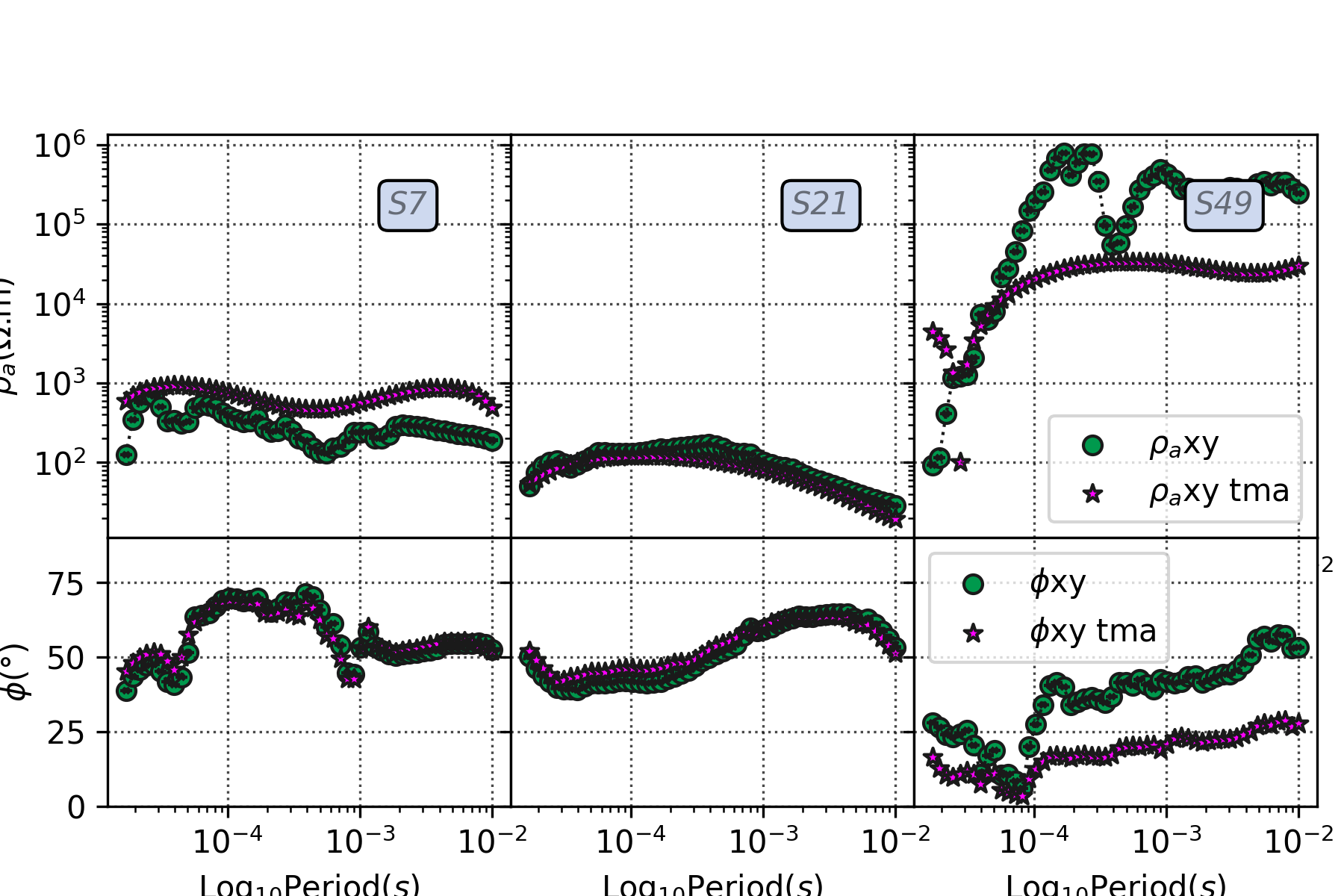
• plot corrections

It is possible to plot correction data using the EMAP filters such as ['tma'| 'ama'|'flma'] or using the static shift (ss) or distorsion (dist) filters. Note that when dist is passed the distorsion must be be provided as 2x2 matrix.

tplot.plot_corrections ( sites = ['s7', 's21', 's49'], fltr ='tma',
                        seed = 52   , markers = ['o', 'd'])# ama is used by default

<'TPlot':survey_area=None, distance=50.0, prefix='S', window_size=5, component='xy', mode='same', method='slinear', out='srho', how='py', c=2>