Plot Receiving Operating Characteristic (ROC)

visualizes the ROC classifier(s) performance.

# Author: L.Kouadio
# Licence: BSD-3-clause

it can plot multiple classifiers at once. If multiple classifiers are given, each classifier must be a tuple of ( <name>, classifier>, <method>). Refer to plotROC()

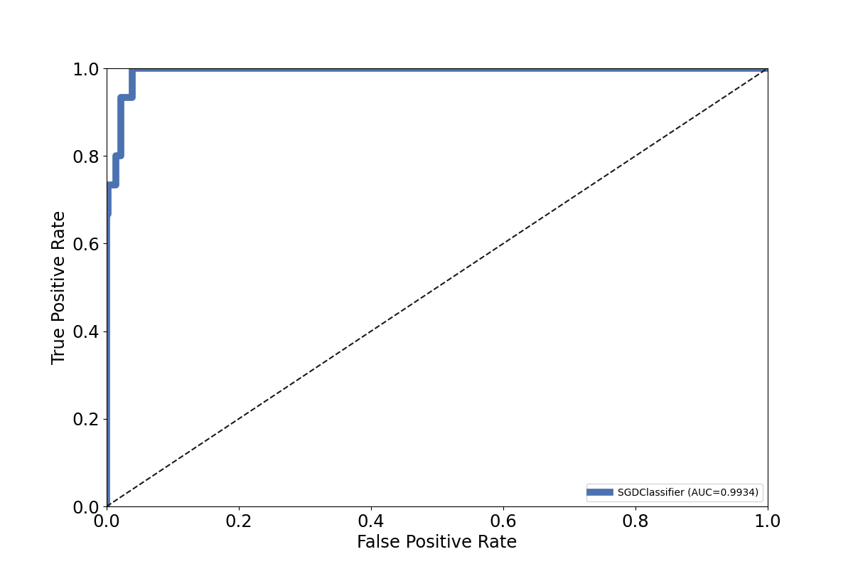
# (1) Plot ROC for single classifier
# note that plot can be customize

from watex.exlib.sklearn import ( SGDClassifier,
                                     RandomForestClassifier
                                     )
from watex.datasets.dload import load_bagoue
from watex.utils import cattarget
from watex.view.mlplot import EvalPlot
X , y = load_bagoue(as_frame =True )
sgd_clf = SGDClassifier(random_state= 42) # our estimator
b= EvalPlot(scale = True , encode_labels=True)
b.lc='b'
b.lw=7
b.font_size =7.
b.fit_transform(X, y)
# binarize the label b.y
ybin = cattarget(b.y, labels= 2 ) # can also use labels =[0, 1]
b.y = ybin
# plot ROC
b.plotROC(sgd_clf , label =1) # class=1

EvalPlot(tname= None, objective= None, scale= True, ... , sns_height= 4.0, sns_aspect= 0.7, verbose= 0)

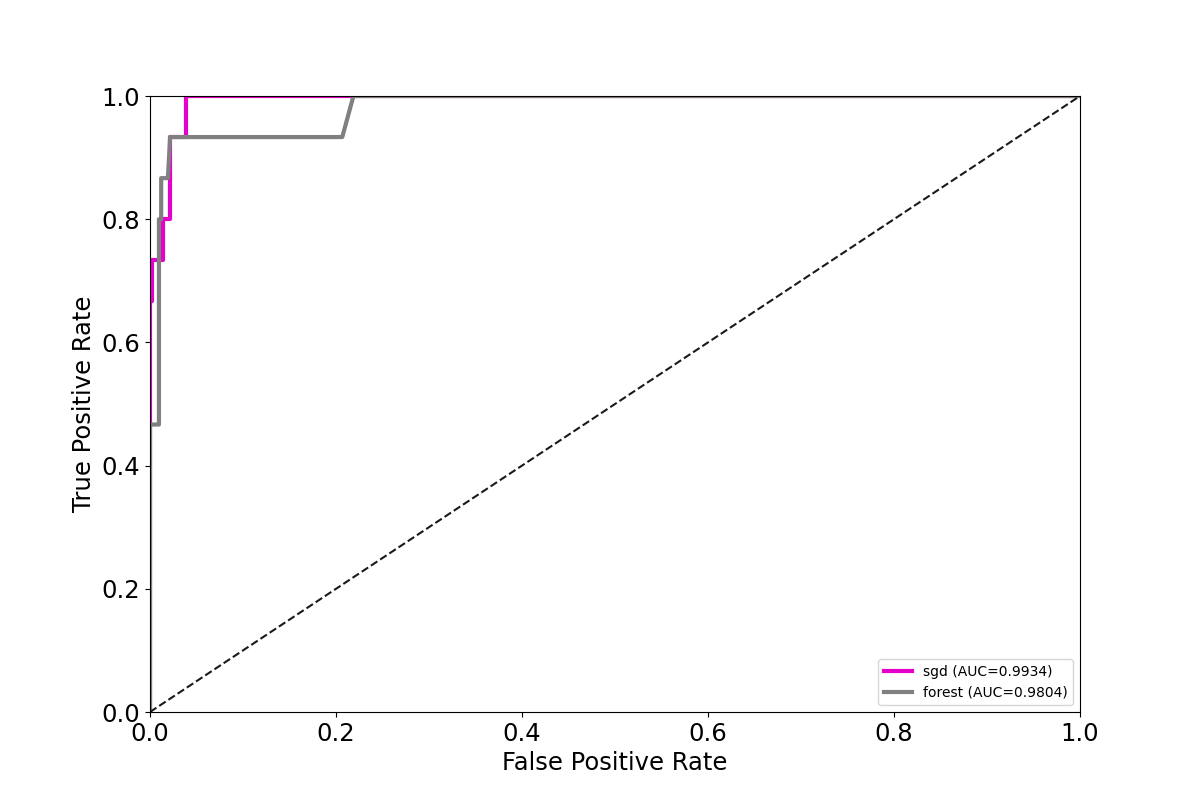
(2)-> Plot ROC for multiple classifiers examples of RandomForest and SDG

b= EvalPlot(scale = True , encode_labels=True,
                lw =3., lc=(.9, 0, .8), font_size=7 )
sgd_clf = SGDClassifier(random_state= 42)
forest_clf =RandomForestClassifier(random_state=42)
b.fit_transform(X, y)
# binarize the label b.y
ybin = cattarget(b.y, labels= 2 ) # can also use labels =[0, 1]
b.y = ybin
clfs =[('sgd', sgd_clf, "decision_function" ),
        ('forest', forest_clf, "predict_proba")]
b.plotROC (clfs =clfs , label =1 )

EvalPlot(tname= None, objective= None, scale= True, ... , sns_height= 4.0, sns_aspect= 0.7, verbose= 0)