Plot apparent resistivity curves

Plot station/site apparent resistivity curves

# Author: L.Kouadio
# Licence: BSD-3-clause

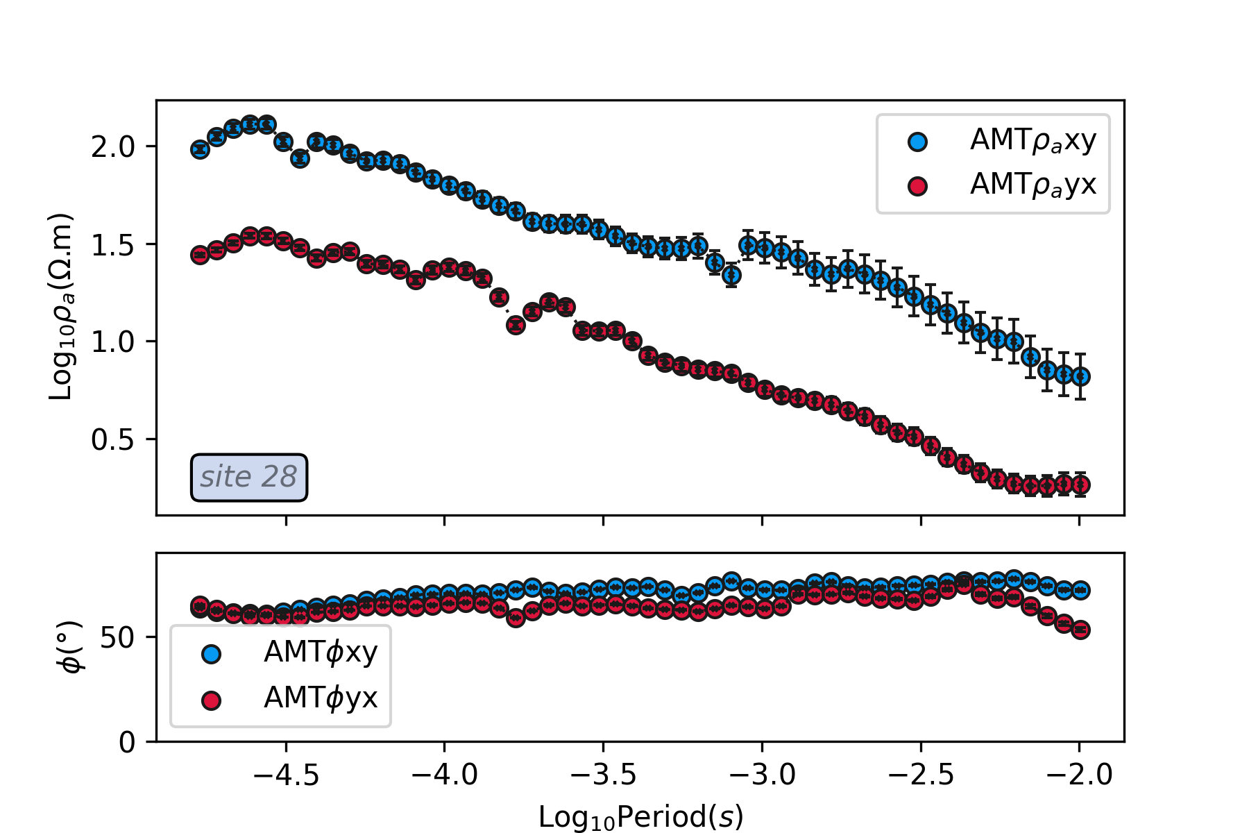
An example of plot apparent resistivity curves with error bar of EDI data collected in Huayaun province. seed is used to reproduce the data at the same station

import watex
test_data = watex.fetch_data ('huayuan', return_data =True , clear_cache=True )
tplot = watex.TPlot(fig_size =(6,  4), marker ='o').fit(test_data)
tplot.plt_style='classic'
tplot.plot_rhoa (seed =52, mode ='*', survey='AMT', show_site =True )

<'TPlot':survey_area=None, distance=50.0, prefix='S', window_size=5, component='xy', mode='same', method='slinear', out='srho', how='py', c=2>

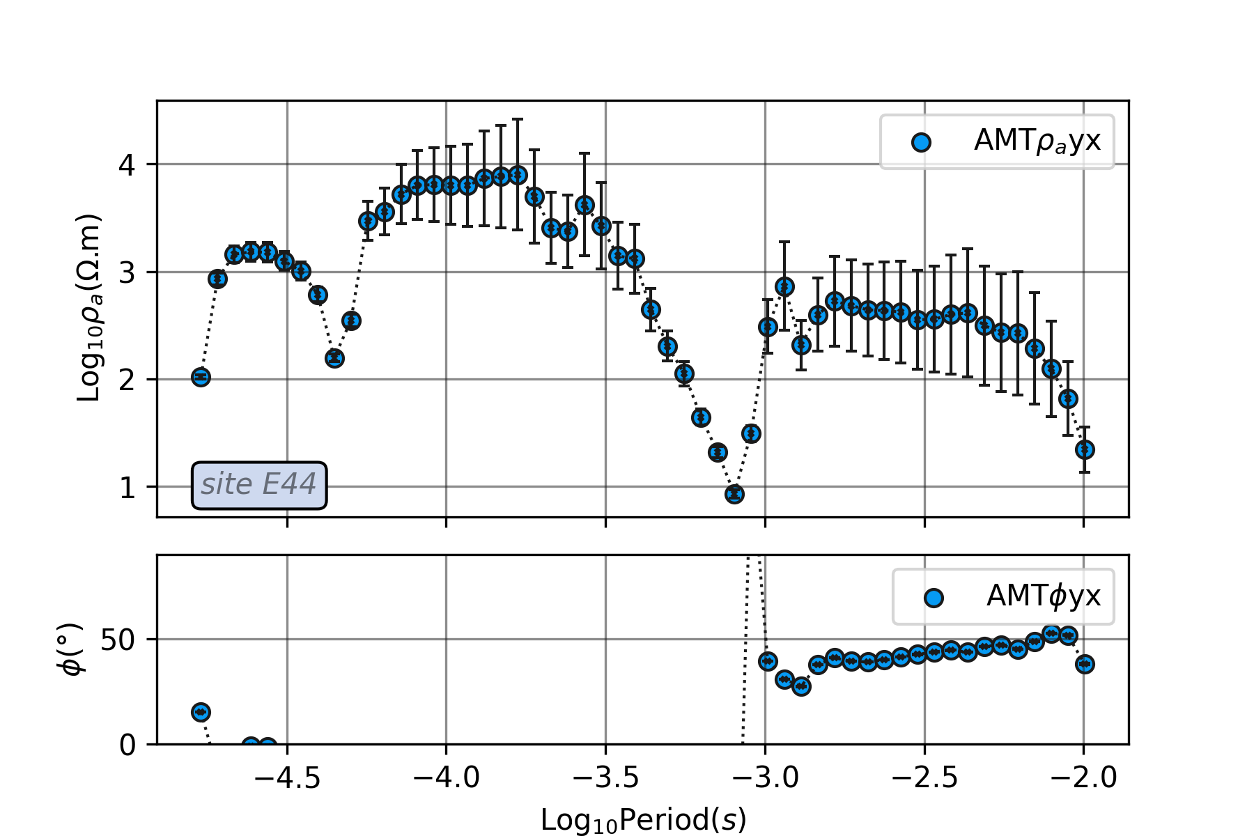
To plot a station data with no errorbar and a single component, we can set, errobar=False and specify the EM mode. For instance, we use the transverse electric mode TE for this example at station s44.

tplot.show_grid=True
tplot.plot_rhoa (site= 'E44', mode ='TM',survey='AMT', show_site =True ,

                )

<'TPlot':survey_area=None, distance=50.0, prefix='S', window_size=5, component='xy', mode='same', method='slinear', out='srho', how='py', c=2>