Plot robust principal components analysis (PCA)

visualizes the robust PCA component analysis from hydro-geological data

# Author: L.Kouadio
# Licence: BSD-3-clause

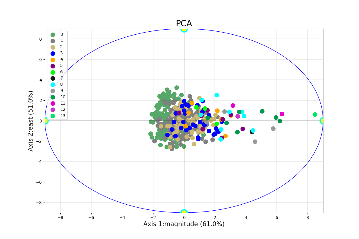
Visualize the first two components PC1 and PC2

from watex.datasets import load_bagoue
from watex.view.mlplot import EvalPlot
X , y = load_bagoue(as_frame =True )
b=EvalPlot(tname ='flow', encode_labels=True ,
                          scale = True )
b.fit_transform (X, y)
b.plotPCA (n_components= 2 )
# Note that pc1 and pc2 labels > n_components -> otherwise  raises user warnings
# Axis 1 and 2 is the default behaviour.
# Runing the script below shows the same figure as the above.

# b.plotPCA (n_components= 2 , biplot=False, pc1_label='Axis 1',
#                       pc2_label='axis 2')
# UserWarning: Number of components and axes might be consistent;
# '2'and '4 are given; default two components are used.

EvalPlot(tname= flow, objective= None, scale= True, ... , sns_height= 4.0, sns_aspect= 0.7, verbose= 0)

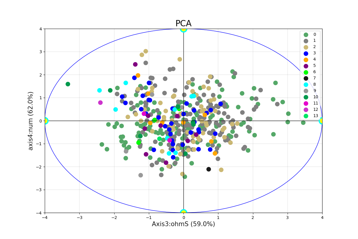
can visulizalise the other components axis in Axis 3 and 4. Note for PC1 and PC2 labels must be consistent with the number of components.

b.plotPCA (n_components= 8 , biplot=False, pc1_label='Axis3',
                         pc2_label='axis4')
# # works fine since n_components are greater to the number of axes

EvalPlot(tname= flow, objective= None, scale= True, ... , sns_height= 4.0, sns_aspect= 0.7, verbose= 0)