2. Base Assessors and Estimators#
The following module is a set of classes and methods composed assessors ( Data
and Missing) and inner-learners or estimators. The `assessors are used for basic controls of the data
whereas the inner-learners are prediction algorithms implemented by watex. In the following, the target value is
expected to be a linear combination of the features. In mathematical notation, if \(\hat{y}\) is the predicted value,
Idem, we designate the vector \(w = (w_1,..., w_p)\) as coef_
and \(w_0\) as intercept_ accross the module.
2.1. Data#
Data is an assessor that can be considered as a shadow class for base data transformation/manipulation. Typically, we train a model with a matrix of data.
Note that pandas dataframe is the most used because it is very nice to have column labels even though
Numpy arrays work as well. For supervised Learning, for instance, such as regression or classification, we
intend to have a function that transforms features into a label. If we were to write this as an algebra formula,
it would look like this:
X is a matrix. Each row represents a sample of data or information about an individual.
Every column in X is a feature. The output of y, is a vector that contains labels
(for classification)or values (for regression). In Python, by convention, we use the variable
name X to hold the sample data even though the capitalization of the variable is a violation
of the standard naming convention (see PEP8).
Data will take in its fit method arrays \(X\) and each column that
composes the dataset can be retrieved as a member:
>>> from watex.base import Data
>>> import pandas as pd
>>> import numpy as np
>>> d = pd.DataFrame ({'a':np.arange (3), 'b':['banana', 'onion', 'apple'], 'c':['obj1','obj2', 'obj3'] })
>>> data= Data().fit(d)
>>> data.a
    0    0
    1    1
    2    2
Name: a, dtype: object
>>> data.b
0     banana
    1     onion
    2     apple
    Name: b, dtype: object
>>> data.shrunk (columns =['b', 'c'])
            b     c
    0  banana  obj1
    1   onion  obj2
    2   apple  obj3
2.2. Missing#
Missing inherits from Data class. It is the second assessor for missing data handling. Indeed, most algorithms will not
work with missing data. As with many things in machine learning, there are no hard answers for
how to treat missing data. Also, missing data could represent different situations. There are
three various ways to handle missing data:
Remove any row with missing data
Remove any columns with missing data
Impute missing values
Create an indicator column to indicate that data was missing
Missing inherits from Data and use missingno. Install the package
missingno for taking advantage of many missing plots. The parameter kind is passed
to Missing for selecting the kind of plot for visualization:
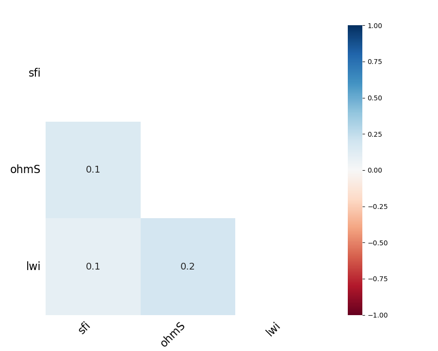
barplot counts the non-missing data using pandasmbaruses themsnopackage to count the number of non-missing data.dendrogramshow the clusterings of where the data is missing. leaves that are the same level predict one onother presence (empty of filled). The vertical arms are used to indicate how different cluster are. short arms mean that branch are similar.corrcreates a heat map showing if there are correlations where the data is missing. In this case, it does look like the locations where missing data are corollated.Noneis the default visualization. It is useful for viewing the contiguous area of the missing data, indicating that the missing data is not random. Thematrixfunction includes a sparkline along the right side. Patterns here would also indicate non-random missing data. It is recommended to limit the number of samples to be able to see the patterns.
Any other value will raise an error. For instance:
>>> from watex.base import Missing
>>> data ='data/geodata/main.bagciv.data.csv'
>>> ms= Missing().fit(data)
>>> # Check the mean values  in the data  in percentage
>>> ms.isnull
num          0.000000
name         0.000000
east         0.000000
north        0.000000
power        0.000000
magnitude    0.000000
shape        0.000000
type         0.000000
sfi          0.013921
ohmS         0.016241
lwi          0.032483
geol         0.000000
flow         0.000000
dtype: float64
>>> ms.kind='corr'
>>> ms.plot(figsize = (12, 4 ))
The corr argument passed to parameter kind output the following picture:
2.3. Sequential Backward Selection#
Sequential Backward Selection (SBS) is a feature selection algorithm that aims to reduce the dimensionality of the initial feature subspace with a minimum decay in the performance of the classifier to improve upon computational efficiency. In certain cases, SBS can even improve the model’s predictive power if a model suffers from overfitting.
Mathematical details
The idea behind the SBS is simple: it sequentially removes features from the full feature subset until the new feature subspace contains the desired number of features. To determine which feature is to be removed at each stage, the criterion function \(J\) is needed for minimization [1]. Indeed, the criterion calculated from the criteria function can simply be the difference in the performance of the classifier before and after the removal of this particular feature. Then, the feature to be removed at each stage can simply be defined as the feature that maximizes this criterion; or in more simple terms, at each stage, the feature that causes the least performance is eliminated loss after removal. Based on the preceding definition of SBS, the algorithm can be outlined with a few steps:
Initialize the algorithm with \(k=d\), where \(d\) is the dimensionality of the full feature space, \(X_d\).
Determine the feature \(x^{-}\),that maximizes the criterion: \(x^{-}= argmax J(X_k-x)\), where \(x\in X_k\).
Remove the feature \(x^{-}\) from the feature set \(X_{k+1}= X_k -x^{-}; k=k-1\).
Terminate if \(k\) equals the number of desired features; otherwise, go to step 2. [2]
>>> from watex.exlib.sklearn import KNeighborsClassifier, train_test_split
>>> from watex.datasets import fetch_data
>>> from watex.base import SequentialBackwardSelection
>>> X, y = fetch_data('bagoue analysed') # data already standardized
>>> Xtrain, Xt, ytrain,  yt = train_test_split(X, y)
>>> knn = KNeighborsClassifier(n_neighbors=5)
>>> sbs= SequentialBackwardSelection (knn)
>>> sbs.fit(Xtrain, ytrain )
2.4. Greedy Perceptron#
Inspired by Rosenblatt’s concept of perceptron rules. Rosenblatt proposed an algorithm that would automatically learn the optimal weights coefficients that would then be multiplied by the input features to decide whether a neuron fires (transmits a signal) or not [3]. In the context of supervised learning and classification, such algorithms could then be used to predict whether a new data point belongs to one class or the other [4]. Rosenblatt’s initial perceptron rule and the perceptron algorithm can be summarized by the following steps:
initialize the weights at 0 or small random numbers.
- For each training examples, \(x^{(i)}\) :
Compute the output value \(\hat{y}\) .
update the weighs.
The weight \(w\) vector can be formally written as:
    >>> from watex.datasets import fetch_data
    >>> from watex.base import GreedyPerceptron
    >>> # Get the spare prepared data
    >>> X, y = fetch_data ('bagoue prepared data')
    >>> GreedyPerceptron ().fit(X.toarray(), y)
GreedyPerceptron(eta=0.01, n_iter=50, random_state=42)
2.5. Majority Vote Classifier#
A majority vote Ensemble classifier combines different classification algorithms associated with individual weights for confidence. The goal is to build a stronger meta-classifier that balance out the individual classifier weaknesses on particular datasets. In more precise mathematical terms, the weighs majority vote can be expressed as follow:
where \(w_j\) is a weight associated with a base classifier, \(C_j\) ; \(\hat{y}\) is the predicted class label of the ensemble. \(A\) is the set of the unique class label; \(\chi_A\) is the characteristic function or indicator function which returns 1 if the predicted class of the jth classifier matches \(i (C_j(x)=1)\). For equal weights, the equation is simplified as follows:
>>> from watex.exlib.sklearn import (
    LogisticRegression,DecisionTreeClassifier ,KNeighborsClassifier,
     Pipeline , cross_val_score , train_test_split , StandardScaler ,
     SimpleImputer )
>>> from watex.datasets import fetch_data
>>> from watex.base import MajorityVoteClassifier
>>> from watex.base import selectfeatures
>>> data = fetch_data('bagoue original').get('data=dfy1')
>>> X0 = data.iloc [:, :-1]; y0 = data ['flow'].values
>>> # exclude the categorical value for demonstration
>>> # binarize the target y
>>> y = np.asarray (list(map (lambda x: 0 if x<=1 else 1, y0)))
>>> X = selectfeatures (X0, include ='number')
>>> X = SimpleImputer().fit_transform (X)
>>> X, Xt , y, yt = train_test_split(X, y)
>>> clf1 = LogisticRegression(penalty ='l2', solver ='lbfgs')
>>> clf2= DecisionTreeClassifier(max_depth =1 )
>>> clf3 = KNeighborsClassifier( p =2 , n_neighbors=1)
>>> pipe1 = Pipeline ([('sc', StandardScaler()),
                       ('clf', clf1)])
>>> pipe3 = Pipeline ([('sc', StandardScaler()),
                       ('clf', clf3)])
Test each classifier’s results taking them individually
>>> clf_labels =['Logit', 'DTC', 'KNN']
>>> # test the results without using the MajorityVoteClassifier
>>> for clf , label in zip ([pipe1, clf2, pipe3], clf_labels):
        scores = cross_val_score(clf, X, y , cv=10 , scoring ='roc_auc')
        print("ROC AUC: %.2f (+/- %.2f) [%s]" %(scores.mean(),
                                                 scores.std(),
                                                 label))
ROC AUC: 0.91 (+/- 0.05) [Logit]
ROC AUC: 0.73 (+/- 0.07) [DTC]
ROC AUC: 0.77 (+/- 0.09) [KNN]
Implement the MajorityVoteClassifier for reducing errors
>>> # test the results with a Majority vote
>>> mv_clf = MajorityVoteClassifier(clfs = [pipe1, clf2, pipe3])
>>> clf_labels += ['Majority voting']
>>> all_clfs = [pipe1, clf2, pipe3, mv_clf]
>>> for clf , label in zip (all_clfs, clf_labels):
        scores = cross_val_score(clf, X, y , cv=10 , scoring ='roc_auc')
        print("ROC AUC: %.2f (+/- %.2f) [%s]" %(scores.mean(),
                                                 scores.std(), label))
... ROC AUC: 0.91 (+/- 0.05) [Logit]
    ROC AUC: 0.73 (+/- 0.07) [DTC]
    ROC AUC: 0.77 (+/- 0.09) [KNN]
    ROC AUC: 0.92 (+/- 0.06) [Majority voting] # give good score & less errors
2.6. Adaline Gradient Descent#
ADAptative LInear NEuron (Adaline) was published by Bernard Widrow [5]. Adaline illustrates the key concepts of defining and minimizing a continuous cost function. This lays the groundwork for understanding more advanced machine learning algorithms for classification, such as Logistic Regression, Support Vector Machines, and Regression models. The key difference between the Adaline rule (also known as the WIdrow-Hoff rule) and Rosenblatt’s perceptron is that the weights are updated based on linear activation function rather than unit step function like in the perceptron. In Adaline, this linear activation function \(\phi(z)\) is simply the identify function of the net input so that:
while the linear activation function is used for learning the weights.
>>> from watex.base import AdalineGradientDescent
>>> from watex.datasets import fetch_data
>>> X, y = fetch_data ('bagoue prepared data')
>>> agd= AdalineGradientDescent ().fit(X.toarray(), y)
>>> agd.w_ # get the weight
    array([-1.18921402e+40,  7.28164687e+39,  7.98336232e+39,  5.04024942e+39,
   -6.58883438e+38,  1.78115247e+39, -1.11444526e+39, -2.27145085e+38,
   -5.63263926e+38, -9.01672565e+39, -9.70560276e+38, -8.14116123e+38,
   -4.94165488e+39, -2.50553865e+39, -3.63083055e+39, -1.91242066e+39,
   -9.13860425e+38, -8.17257230e+39, -8.93286811e+38])
2.7. Adaline Gradient Descent with Batch#
Adaptative Linear Neuron Classifier with batch (stochastic) gradient descent ( AdalineStochasticGradientDescent )
is a popular alternative which is sometimes also called iterative or online gradient descent. Here,
weights are updated based on the sum of accumulated errors over all training examples \(x^{(i)}\):
the weights are updated incrementally for each training example:
>>> from watex.base import AdalineStochasticGradientDescent
>>> from watex.datasets import fetch_data
>>> X, y = fetch_data ('bagoue prepared data')
>>> asgd =AdalineStochasticGradientDescent ().fit(X.toarray(), y)
array([ 0.00496714,  0.50482389,  0.08465044,  0.14398117, -0.01095346,
                0.11365574,  0.4715504 ,  0.65265459,  0.27175669,  0.4257843 ,
                0.52242138,  0.48250745,  0.58282695,  0.52649733,  0.69415282,
                0.56346338,  0.62798868,  0.45071501,  0.66074818])